Introduction

The autoregressive process are one of the most simple models studied in coursed or time series analysis. An interessante feature of autoregressive process is their similar with linear regression models. For instance, the firs order autoregressive, \(\mathrm{AR}(1)\), can be definied as follows: \[\begin{equation}\label{eq:ar1} Y_t \sim N(\mu_t, \sigma^2), \quad \text{where} \quad \mu_t = \alpha + \phi\,y_{t-1} \end{equation}\] for \(t = 1,\ldots,n\). Note that \(y_{t-1}\) play the role of covariate and the variance is constant along time.

The goal of this post is to show a naive implementation in R for simulation, esitmatiopn and forecasting an \(\mathrm{AR}(1)\) model. Although it is already available thought the functions arima.sim() and arima() this exercise provides a understanding of model structure, and consequently a path to more complex model implementations.

Simulation

Let us consider the true parameter values as \(\alpha = -2.0\), \(\phi = 0.7\), \(\sigma^2 = 4.0\) and the sample size \(n = 500\). Since the probability distribution of the \(Y_t\) is Normal I will use rnorm() function.

set.seed(666)
n <- 500
alpha <- -2.0
sigma <- 2.0
phi <- 0.7
y <- numeric(n)
for(t in 2:n) {
  mu_t <- alpha + phi * y[t-1]
  y[t] <- rnorm(1, mean = mu_t, sd = sigma)
}
ts.plot(y)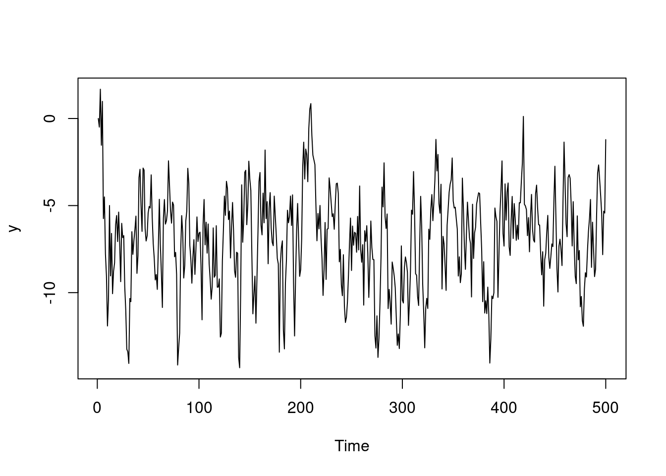

Estimation

Given a random sample \(\mathbf{y} = (y_1, \ldots, y_n)\) of the model \(\mathrm{AR}(1)\), under normality assumption the likelihood is given by \[ L(\mathbf{\theta} \mid \mathbf{y}) \propto (\sigma^2)^{-\frac{n}{2}}\,\exp\left\{-\frac{1}{2\,\sigma^2}\sum_{t=2}^{n}\left[y_t - (\alpha -\phi\,y_{t-1}) \right]^2 \right\} \] where \(\mathbf{\theta} = (\alpha, \phi, \sigma^2)\).

The maximum likelihood estimates of parameter vector \(\mathbf{\theta}\) is obtained by the maximization of the log-likelihood.

log_like <- function(parms, y) {
  n <- length(y)

  phi <- parms[1]
  alpha <- parms[2]
  sigma <- parms[3]

  eta <- numeric(n)

  for(k in 2:n) eta[k] <- phi * y[k-1]

  ll <- sum(dnorm(x = y, mean = eta + alpha, sd = sigma, log = TRUE))
  ll
}

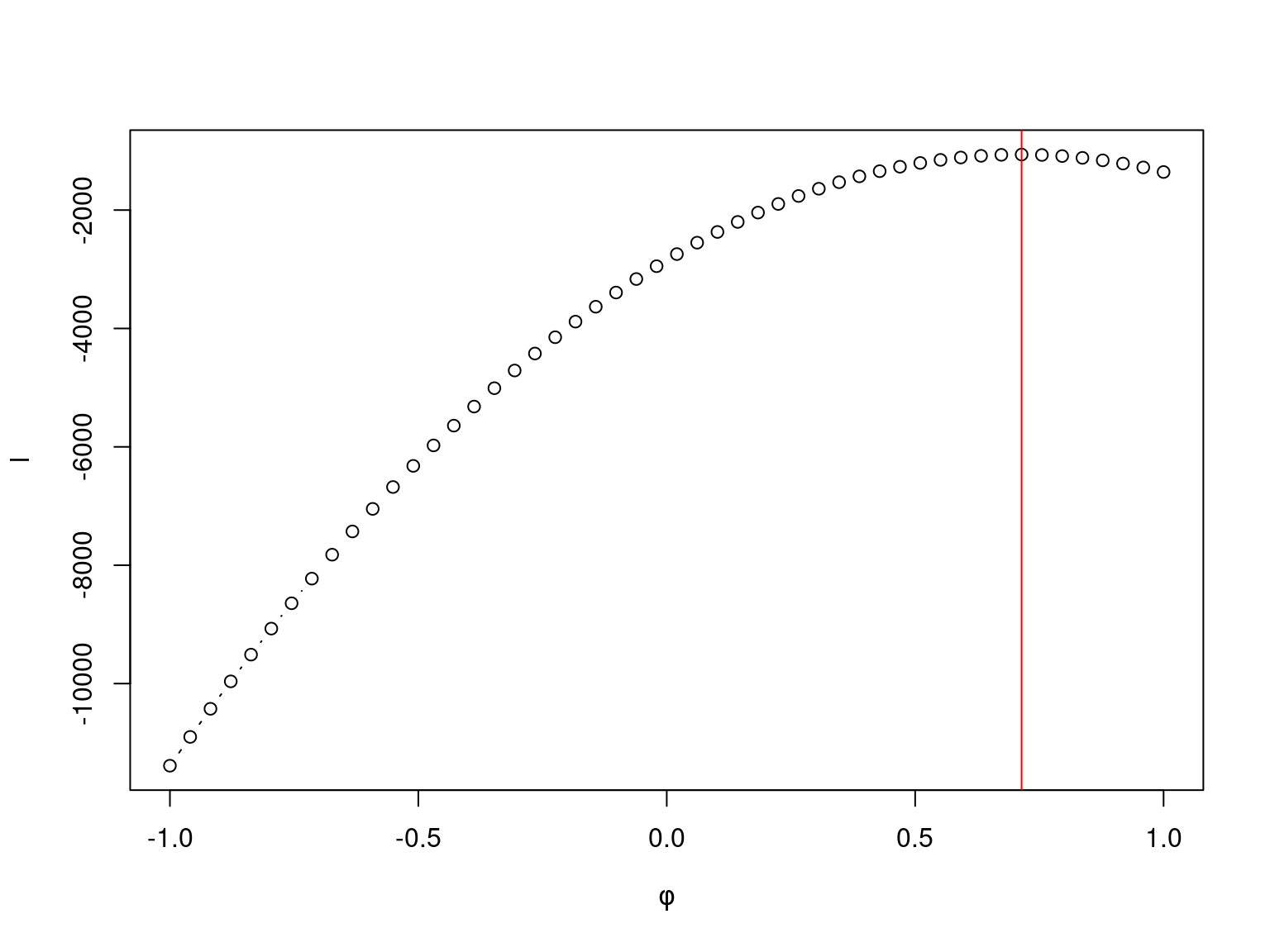
For fixed values of \(\alpha\) and \(\sigma^2\) the profile likelihood of \(\phi\) for the simulated data has the follwing behaviour

The numeric maximization of log-likelihood in R is performed by the optim function. I use the quasi-newton BFGS optimization algorithm (method = "BFGS"), I stated to maximize the function by using control = list(fnscale = -1) and requested to compute the numerical hessian (hessian = TRUE).

fit <- optim(par = c(phi, alpha, sigma), fn = log_like, y = y, method = "BFGS",
             control = list(fnscale = -1), hessian = TRUE)

The paramter estimated for \(\phi\), \(\alpha\), and \(\sigma\) are, respectively,

## [1]  0.6997547 -2.0902103  2.0239194

Very close to the true values:

## [1]  0.7 -2.0  2.0

Note that the eigenvalues of hessian matriz are negatives, then such estimates are in fact the maximum likelihood estimates.

eigen(fit$hessian)$values

## [1]   -17.22736  -244.12550 -6993.97570

Forecast

For the \(\mathrm{AR}(1)\) model the forecast value at time \(t\) is given by

\[ y_{t} = \hat{\alpha} + \hat{\phi}\,y_{t-1} \] where \(\hat{\alpha}\) and \(\hat{\phi}\) are the maximum likelihood estimates of \(\alpha\) and \(\phi\), respectively.

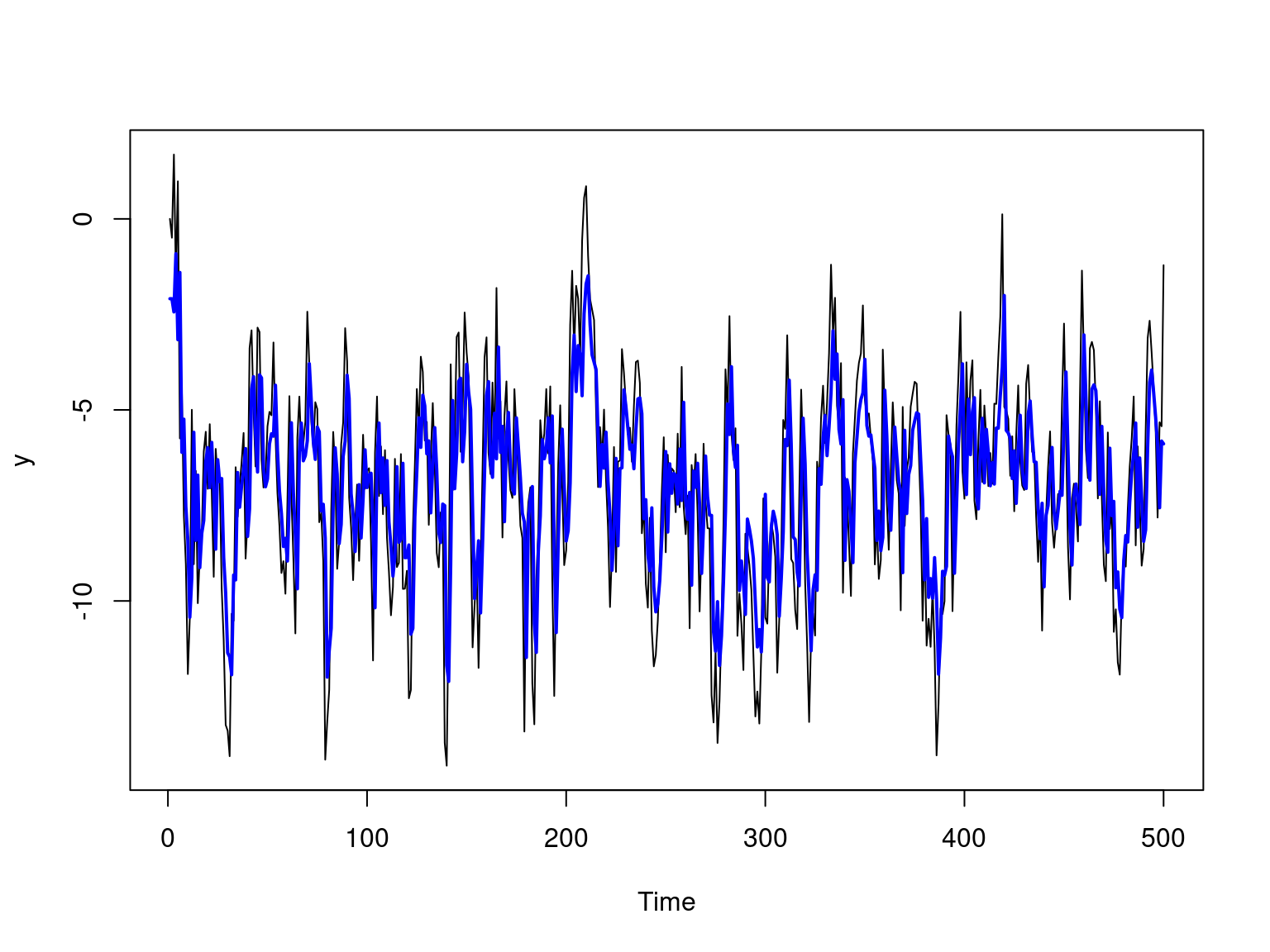
The picture below shows the simulated time series and the forecast values of \(\mathrm{AR}(1)\) model.

mles <- fit$par
phi_hat <- mles[1]
alpha_hat <- mles[2]
sigma_hat <- mles[3]
yhat <- numeric(n)
for(t in 2:n) yhat[t] <- phi_hat * y[t-1]
ts.plot(y)
lines(yhat + alpha_hat, type = "l", col = "blue", lwd = 2)