The problem

The Expectation and Maximization (EM) algorithm is a general procedure to find the maximum likelihood estimates when the phenomena of interest is describe by a model with missing values or latent variables.

In this post I will discus the EM algorithm thorough the following example. Assume that we observe \(X_1, \ldots, X_n\) and know that \[ X_i = I_{\left\{Z_i > r\right\}} = \begin{cases} 1 & \textrm{if } Z_i > r \\ 0 & \textrm{if } Z_i \leq r \end{cases} \] where \(r\) is known and \(Z_i \sim N(\mu, \sigma^2) \quad \forall\, i=1, \ldots, n\) are unknown.

The problem is, how can we estimate the parameters \(\boldsymbol{\theta} = (\mu, \sigma^2)\) using the observed values \(\boldsymbol{x} = (x_1, \ldots, x_n)\) from the random variables \(\mathbf{X} = (X_1, \ldots, X_n)\)?

Solution

First, note that \(X_i \sim \textrm{Bernoulli}(p)\) where the probability of success is \[ p = P(X_i = 1) = P(Z_i > r) = 1 - \varPhi(r) \] where \(\varPhi(\cdot)\) is the c.d.f. of standard Normal distribution defined as \[ \varPhi(x) = \int_{-\infty}^{x} \varphi(t) \mathrm{d}t \quad \text{e} \quad \varphi(x) = \dfrac{1}{\sqrt{2 \pi} \sigma} \mathrm{e}^{- \dfrac{(x - \mu)^2}{2\sigma^2}}. \]

To use the EM algorithm we need to find the complete likelihood, that is the joint distribution of \((\mathbf{X}, \mathbf{Z}) \sim f(\boldsymbol{x}, \boldsymbol{z})\). Using conditional probability arguments we can write the joint distribution for a single observation as \[ f_{X_i, Z_i}(x, z) = f_{Z_i \mid X_i = x}(z \mid x) f_{X_i}(x). \]

We also know that \[ f_{X_i}(x) = \left[1 - \varPhi\left(r\right)\right]^{x} \left[\varPhi\left(r\right) \right]^{1 - x},\, \quad \mathrm{para}\, x = 0, 1. \]

In addition, an important remark is that \(Z_i \mid X_i = x_i\) follows a Bernoulli distribution where the probability of success is given by a truncated Normal distribution at \(r\). Its p.d.f. can be written as \[ f_{Z_i \mid X_i = x}(z_i \mid x_i) = \left[\dfrac{\varphi(z_i)}{1 - \varPhi(r)}\right]^{x_i}\,\left[\dfrac{\varphi(z_i)}{\varPhi(r)}\right]^{1 - x_i}, \, \quad x_i = 0, 1. \]

Hence, the joint distribution of \((X_i, Z_i)\) is given by \[ f_{X_i, Z_i}(x_i, z_i) = \left[\dfrac{\varphi(z_i)}{1 - \varPhi(r)}\right]^{x_i}\,\left[\dfrac{\varphi(z_i)}{\varPhi(r)}\right]^{1 - x_i}\, \left[1 - \varPhi\left(r\right)\right]^{x_i} \left[\varPhi\left(r\right) \right]^{1 - x_i} = \varphi(z_i). \]

And the complete likelihood for a sample of size \(n\) is given by \[ L_c(\boldsymbol{\theta} \mid \boldsymbol{z}, \boldsymbol{x}) = \prod_{i=1}^n \varphi(z_i) = \left(2 \pi \sigma^2\right)^{-n/2}\,\exp\left\{-\dfrac{1}{2\sigma^2}\,\sum_{i=1}^n (z_i - \mu)^2\right\} \] where \(\boldsymbol{\theta} = (\mu, \sigma^2)\)

The E step of EM algorithm is to calculate the expectation of the log-likelihood with respect to the distribution of \((Z_i \mid X_i = x_i)\). Given an initial value \(\boldsymbol{\theta}_0 = (\mu_0, \sigma^2_0)\) we have \[ \begin{eqnarray} Q(\boldsymbol{\theta} \mid \boldsymbol{\theta}_0, \boldsymbol{x}) &=& -\dfrac{n}{2}\log(2 \pi \sigma^2) - \dfrac{1}{2\,\sigma^2}\sum_{i=1}^n\left[ \mathbb{E}(Z_i^2 \mid x_i, \boldsymbol{\theta}_0) - 2 \mu \mathbb{E}(Z_i \mid x_i, \boldsymbol{\theta}_0) + \mu^2 \right] \nonumber \\ \nonumber &=& -\dfrac{n}{2}\log(2 \pi \sigma^2) - \dfrac{1}{2\,\sigma^2}\left[\sum_{i=1}^n h_i(\boldsymbol{\theta}_0) - 2 \mu \sum_{i=1}^n k_i(\boldsymbol{\theta}_0) + n\,\mu^2\right]. \end{eqnarray} \] where \(k_i(\boldsymbol{\theta}_0) = \mathbb{E}(Z_i \mid x_i, \boldsymbol{\theta}_0)\) and \(h_i(\boldsymbol{\theta}_0) =\mathbb{E}(Z_i^2 \mid x_i, \boldsymbol{\theta}_0)\).

Now, in the M step we should maximize \(Q(\boldsymbol{\theta} \mid \boldsymbol{\theta}_0, \boldsymbol{x})\). Note that

\[ \begin{eqnarray} \dfrac{\partial}{\partial \mu} Q(\boldsymbol{\theta} \mid \boldsymbol{\theta}_0, \boldsymbol{x}) &=& -\dfrac{1}{2\,\sigma^2}\left[2 \sum_{i=1}^n k_i(\boldsymbol{\theta}_0) + 2n\mu\right] \label{eq:mu} \\ \label{eq:sigma2} \dfrac{\partial}{\partial \sigma^2} Q(\boldsymbol{\theta} \mid \boldsymbol{\theta}_0, \boldsymbol{x}) &=& -\dfrac{n}{2 \sigma^2} + \dfrac{1}{2\,(\sigma^2)^2}\left[\sum_{i=1}^n h_i(\boldsymbol{\theta}_0) - 2 \mu \sum_{i=1}^n k_i(\boldsymbol{\theta}_0) + n\,\mu^2\right]. \end{eqnarray} \]

Setting the above equations to zero and solving for \(\mu\) and \(\sigma^2\) it turns out that \[ \begin{eqnarray} \dfrac{\partial}{\partial \mu} Q(\boldsymbol{\theta} \mid \boldsymbol{\theta}_0, \boldsymbol{x}) = 0 &\rightarrow& \widehat{\mu} = \dfrac{1}{n} \sum_{i=1}^n k_i(\boldsymbol{\theta}_0) \\ \dfrac{\partial}{\partial \sigma^2} Q(\boldsymbol{\theta} \mid \boldsymbol{\theta}_0, \boldsymbol{x}) = 0 &\rightarrow& \widehat{\sigma}^2 = \dfrac{1}{n}\left[\sum_{i=1}^n h_i(\boldsymbol{\theta}_0) - 2 \widehat{\mu} \sum_{i=1}^n k_i(\boldsymbol{\theta}_0) + n\,\widehat{\mu}^2\right] \rightarrow \nonumber \\ &\rightarrow& \widehat{\sigma}^2 = \dfrac{1}{n}\left[\sum_{i=1}^n h_i(\boldsymbol{\theta}_0) - \dfrac{1}{n}\left(\sum_{i=1}^n k_i(\boldsymbol{\theta}_0)\right)^2 \right]. \end{eqnarray} \] Now, we should find the expectations, i.e., \(k_i(\boldsymbol{\theta}_0) = \mathbb{E}(Z_i \mid x_i, \boldsymbol{\theta}_0)\) and \(h_i(\boldsymbol{\theta}_0) =\mathbb{E}(Z_i^2 \mid x_i, \boldsymbol{\theta}_0)\). Remembering that \((Z_i \mid X_i = x_i)\) has Bernoulli distribution with the probability of success being a truncated Normal distribution at \(r\). Thus, for \(Z_i \mid X_i = 1\) the moment generating function is

\[ \begin{align*} M_{Z_i \mid X_i = 1}(t) = \mathbb{E}[\mathrm{e}^{t Z}] & = \dfrac{1}{1-\varPhi(r)} \int_r^{\infty} \mathrm{e}^{tz} \phi(z)\mathrm{d}z = \dfrac{1}{1-\varPhi(r)} \int_r^{\infty} \mathrm{e}^{tz} \dfrac{1}{\sqrt{2 \pi} \sigma} \mathrm{e}^{- \dfrac{(z - \mu)^2}{2\sigma^2}}\mathrm{d}z\\ \\ &= \exp\left\{\mu t+ \sigma^2 t^2 / 2 \right\}\,\dfrac{1 - \varPhi(r - \sigma t)}{1 - \varPhi(r)}. \end{align*} \] On the other hand, the moment generating function of \(Z_i \mid X_i = 1\) is

\[ \begin{align*} M(t) = \mathbb{E}[\mathrm{e}^{t Z}] & = \dfrac{1}{\varPhi(r)} \int_{-\infty}^r \mathrm{e}^{tz} \phi(z)\mathrm{d}z = \dfrac{1}{\varPhi(r)} \int_{-\infty}^r \mathrm{e}^{tz} \dfrac{1}{\sqrt{2 \pi} \sigma} \mathrm{e}^{- \dfrac{(z - \mu)^2}{2\sigma^2}}\mathrm{d}z\\ \\ &= \exp\left\{\mu t+ \sigma^2 t^2 / 2 \right\}\,\dfrac{\varPhi(r - \sigma t)}{\varPhi(r)}. \end{align*} \] Then the first two moments of \(Z_i \mid X_i = x_i\) are given by

\[ E(Z_i \mid X_i = x_i) = M^{\prime}(t)|_{t=0} = \begin{cases} \mu + \sigma \dfrac{\varphi(r)}{1 - \varPhi(r)}, & \mathrm{if} \, x_i = 1 \\ \\ \mu - \sigma \dfrac{\varphi(r)}{\varPhi(r)}, & \mathrm{if} \, x_i = 0 \end{cases} \] and \[ E(Z^2_i \mid X_i = x_i) = M^{\prime\prime}(t)|_{t=0} = \begin{cases} \mu^2 + \sigma^2 + \sigma(r + \sigma) \dfrac{\varphi(r)}{1 - \varPhi(r)}, & \mathrm{if} \, x_i = 1 \\ \\ \mu^2 + \sigma^2 - \sigma(r + \sigma) \dfrac{\varphi(r)}{\varPhi(r)}, & \mathrm{if} \, x_i = 0. \end{cases} \] Finally, using the expressions of \(k_i(\boldsymbol{\theta}_0)\) and \(h_i(\boldsymbol{\theta}_0)\) we can implement the EM algorithm to estimate \(\boldsymbol{\theta} = (\mu , \sigma^2)\).

In general, the EM steps are the following

1. Given initial guess \(\boldsymbol{\theta}_j = (\mu_j, \sigma_j^2)\);

2. Compute: \[\begin{eqnarray*} \widehat{\mu}_{j+1} &=& \dfrac{1}{n} \sum_{i=1}^n k_i(\boldsymbol{\theta}_{j}) \\ \widehat{\sigma}^2_{j+1} &=& \dfrac{1}{n}\left[\sum_{i=1}^n h_i(\boldsymbol{\theta}_{j}) - \dfrac{1}{n}\left(\sum_{i=1}^n k_i(\boldsymbol{\theta}_j)\right)^2 \right]. \end{eqnarray*}\] and then \(\boldsymbol{\theta}_{j+1} = (\widehat{\mu}_{j+1}, \widehat{\sigma}^2_{j+1})\).

3. If \(\max\left(|\boldsymbol{\theta}_{j} - \boldsymbol{\theta}_{j+1}|\right) < \varepsilon\) then the convergence criteria is satisfied and the EM estimates of \(\boldsymbol{\theta}\) is \(\boldsymbol{\theta}_{j+1}\).

4. Otherwise, update \(\boldsymbol{\theta}_{j}\) for \(\boldsymbol{\theta}_{j+1}\) and go through to step (ii).

It is noteworthy that this is a naive example where the two steps of EM algorithm, the expectation and the maximization can be derived analytically. Generally, this is not the case for more complex problem although it is possible to obtain some sort of approximations.

R implementation

In the sequel an R implementation is presented. First, we need to define a function to compute the first and second moments of the distribution \((Z_i \mid X_i = x_i)\). The below moments function can do that.

moments <- function(x, r, theta) {
  mu <- theta[1]
  sigma2 <- theta[2]
  sigma <- sqrt(sigma2)
  if (x == 1) {
    ki <- mu + sigma * dnorm(r, mu, sigma) / 
      pnorm(r, mu, sigma, lower.tail = F)
    hi <- mu^2 + sigma^2 + sigma * (r + mu) * 
      dnorm(r, mu, sigma) / pnorm(r, mu, sigma, lower.tail = F)
  } else {
    ki <- mu - sigma * dnorm(r, mu, sigma) / 
      pnorm(r, mu, sigma)
    hi <- mu^2 + sigma^2 - sigma * (r + mu) * 
      dnorm(r, mu, sigma) / pnorm(r, mu, sigma)
  }
  c(ki, hi)
}

Then, the EM algorithm is implemented in the expectation_maximization showed in the sequence. Note that for each iteration we keep the estimates of \(\mu\) and \(\sigma^2\). The function returns a matrix with the parameter estimates in each iteration. The algorithm stops when reach out the convergence criteria, which is defined as \[ \max(|\boldsymbol{\theta}_{j} - \boldsymbol{\theta}_{j+1}|) < \epsilon \] where \(\epsilon = 10^{-5}\).

expectation_maximization <- function(x, r, theta, tol = 1e-5) {
  estimates <- list()
  n <- length(x)
  err <- 1
  j <- 0L
  while (err > tol) {
    E <- sapply(x, moments, r = r, theta = theta)
    s_E <- rowSums(E, na.rm = T)  
    mu_j <- 1 / n * s_E[1]
    sigma2_j <- 1 / n * (s_E[2] - 1 / n * (s_E[1])^2)
    err <- max(abs(theta[1] - mu_j), abs(theta[2] - sigma2_j))
    theta <- c(mu_j, sigma2_j)
    j <- j + 1
    estimates[[j]] <- c(j, theta)
  }
  m <- do.call(rbind, estimates)
  colnames(m) <- c("Iteration", "mu", "sigma2")
  m
}

To evaluate the algorithm a simulate example in presented. I simulated \(Z_i \sim N(4, 2)\) and \(r = 4\) then the expectation_maximization is used to get the estimates.

set.seed(69)
z <- rnorm(100, mean = 4, sd = 2)
r <- 4
x <- ifelse(z > r, 1, 0)
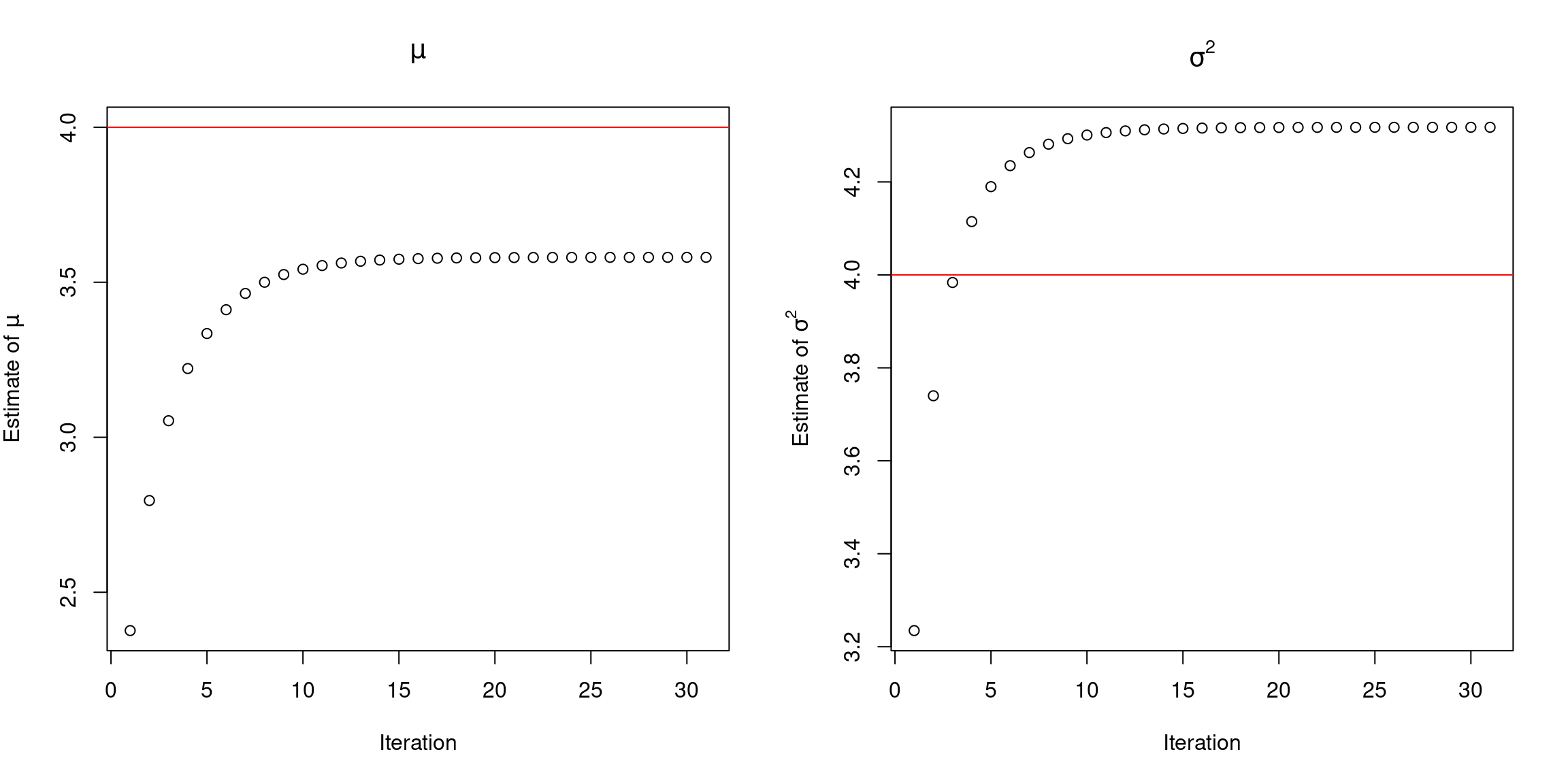
out <- expectation_maximization(x = x, r = r, theta = c(1, 1), tol = 1e-5)

The algorithm reach out the convergence with 31 iteration, and the final estimates of \(\mu\) and \(\sigma^2\) are 3.580 and 4.318, which are close to the true values \(\mu = 4\) and \(\sigma^2 = 4\).

The Figure above shows the estimates obtained in each iteration for the parameters. Interesting to note that the EM estimates for \(\mu\) is underestimate the true value, while for \(\sigma^2\) is overestimate.

par(mfrow = c(1, 2))
plot(out[, 2], ylim = c(min(out[, 2]), 4), main = expression(mu),
     xlab = "Iteration", ylab = bquote("Estimate of"~mu))
abline(h = 4, col = "red")
plot(out[, 3], main = expression(sigma^2),
     xlab = "Iteration", ylab = bquote("Estimate of"~sigma^2))
abline(h = 4, col = "red")