Density function, distribution function, quantile function and random number generation function for the Johnson SB distribution reparametrized in terms of the \(\tau\)-th quantile, \(\tau \in (0, 1)\).
Usage
djohnsonsb(x, mu, theta, tau = 0.5, log = FALSE)

pjohnsonsb(q, mu, theta, tau = 0.5, lower.tail = TRUE, log.p = FALSE)

qjohnsonsb(p, mu, theta, tau = 0.5, lower.tail = TRUE, log.p = FALSE)

rjohnsonsb(n, mu, theta, tau = 0.5)
Arguments
- x, q
vector of positive quantiles.
- mu
location parameter indicating the \(\tau\)-th quantile, \(\tau \in (0, 1)\).
- theta
nonnegative shape parameter.
- tau
the parameter to specify which quantile is to used.
- log, log.p
logical; If TRUE, probabilities p are given as log(p).
- lower.tail
logical; If TRUE, (default), \(P(X \leq{x})\) are returned, otherwise \(P(X > x)\).
- p
vector of probabilities.
- n
number of observations. If
length(n) > 1, the length is taken to be the number required.
Value
djohnsonsb gives the density, pjohnsonsb gives the distribution function,
qjohnsonsb gives the quantile function and rjohnsonsb generates random deviates.
Invalid arguments will return an error message.
Details
Probability density function $$f(y\mid \alpha ,\theta )=\frac{\theta }{\sqrt{2\pi }}\frac{1}{y(1-y)}\exp\left\{ -\frac{1}{2}\left[\alpha +\theta \log\left(\frac{y}{1-y}\right)\right] ^{2}\right\}$$
Cumulative distribution function $$F(y\mid \alpha ,\theta )=\Phi \left[ \alpha +\theta \log \left( \frac{y}{1-y}\right) \right]$$
Quantile function $$Q(\tau \mid \alpha ,\theta )=\frac{\exp \left[ \frac{\Phi ^{-1}(\tau)-\alpha }{\theta }\right] }{1+\exp \left[ \frac{\Phi ^{-1}(\tau )-\alpha }{\theta }\right] }$$
Reparameterization $$\alpha =g^{-1}(\mu )=\Phi ^{-1}(\tau )-\theta \log \left( \frac{\mu }{1-\mu }\right)$$
References
Lemonte, A. J. and Bazán, J. L., (2015). New class of Johnson SB distributions and its associated regression model for rates and proportions. Biometrical Journal, 58(4), 727--746.
Johnson, N. L., (1949). Systems of frequency curves generated by methods of translation. Biometrika, 36(1), 149--176.
Examples
set.seed(123)
x <- rjohnsonsb(n = 1000, mu = 0.5, theta = 1.5, tau = 0.5)
R <- range(x)
S <- seq(from = R[1], to = R[2], by = 0.01)
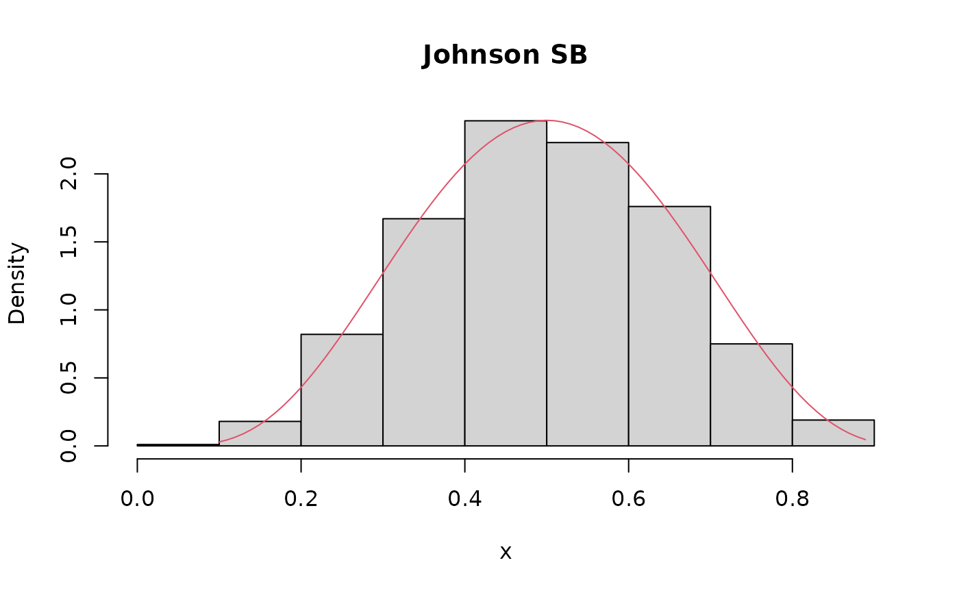
hist(x, prob = TRUE, main = 'Johnson SB')
lines(S, djohnsonsb(x = S, mu = 0.5, theta = 1.5, tau = 0.5), col = 2)
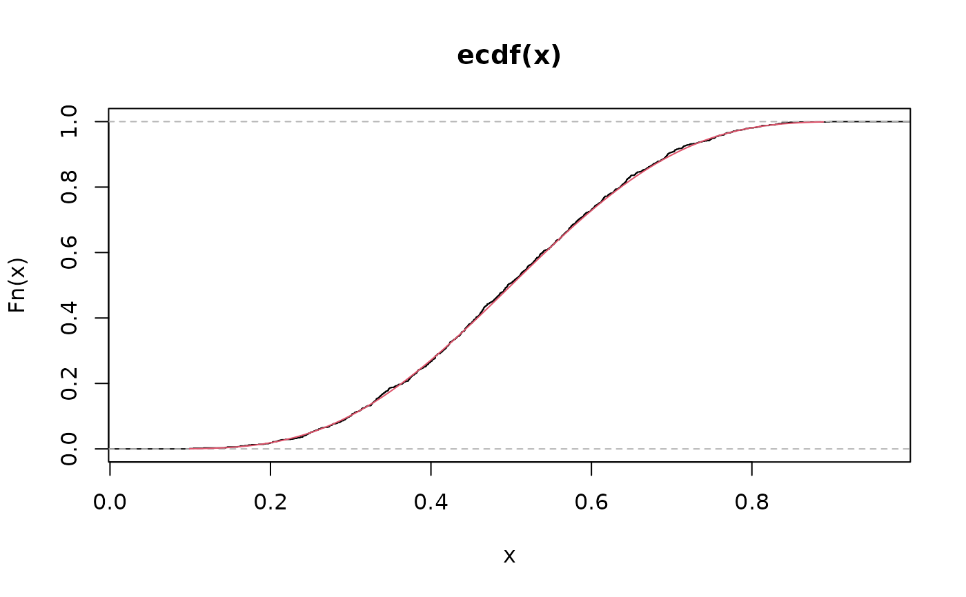
 plot(ecdf(x))
lines(S, pjohnsonsb(q = S, mu = 0.5, theta = 1.5, tau = 0.5), col = 2)
plot(ecdf(x))
lines(S, pjohnsonsb(q = S, mu = 0.5, theta = 1.5, tau = 0.5), col = 2)
 plot(quantile(x, probs = S), type = "l")
lines(qjohnsonsb(p = S, mu = 0.5, theta = 1.5, tau = 0.5), col = 2)
plot(quantile(x, probs = S), type = "l")
lines(qjohnsonsb(p = S, mu = 0.5, theta = 1.5, tau = 0.5), col = 2)