Structure and functionality

Introduction

The unitquantreg R package provide efficient tools for estimation and inference in parametric quantile regression models for bounded data.

The current version of unitquantreg has 11 probability distributions available for user choice. The Table above lists the families of distributions, their abbreviations and the paper reference.

Available families of distributions their abbreviations and reference.
Family	Abbreviation	Reference
arc-secant hyperbolic Weibull	ashw	Korkmaz et al. (2021)
Johnson-SB	johnsonsb	Johnson (1949)
Kumaraswamy	kum	Kumaraswamy, (1980)
log-extended Exponential-Geometric	leeg	Jodrá and Jiménez-Gamero (2020)
unit-Birnbaum-Saunders	ubs	Mazucheli, et al. (2021)
unit-Burr-XII	uburrxii	Korkmaz and Chesneau (2021)
unit-Chen	uchen	Korkmaz, et al. (2020)
unit-Generalized Half-Normal-E	ughne	Korkmaz MÇ (2020)
unit-Generalized Half-Normal-X	ughnx	New
unit-Gompertz	ugompertz	Mazucheli et al. (2019)
unit-Gumbel	ugumbel	New
unit-Logistic	ulogistic	Tadikamalla and Johnson (1982)
unit-Weibull	uweibull	Mazucheli, et al. (2018)

The [dpqr]’s functions of the distributions are vectorized and implemented in C++. The log likelihood, score and hessian functions are also implemented in C++ in order to guarantee more computational efficiency.

The parameter estimation and inference are performed under the frequentist paradigm. Maximization of the log-likelihood function is done by optimization techniques available in the R through the optimx package, which is a general-purpose optimization wrapper function that allows the use of several R tools for optimization, including the existing stats::optim() function. To achieve quick and better convergence the analytical score function is use during the maximization. Also, standard errors of parameter estimates are computed using the analytical hessian matrix.

Structure

The unitquantreg package is built around the unitquantreg() function which perform the fit of parametric quantile regression models via likelihood method. The unitquantreg() function has standard arguments as stats::glm() function, and they are as follows:

#> function (formula, data, subset, na.action, tau, family, link = c("logit", 
#>     "probit", "cloglog", "cauchit"), link.theta = c("identity", 
#>     "log", "sqrt"), start = NULL, control = unitquantreg.control(), 
#>     model = TRUE, x = FALSE, y = TRUE) 
#> NULL

The formula argument use the concept of Formula package allows multiple parts on the right-hand side, which indicates regression structure for the quantile and shape parameter of the distribution. For instance, formula = y ~ x1 | z1 means the following regression structure

\[ g_1(\mu) = \beta_0 + \beta_1\,x_1 \quad \textrm{and} \quad g_2(\theta) = \gamma_0 + \gamma_1\,z_1 \] where \(\mu\) indicates the quantile of order \(\tau\) and \(\theta\) is the shape parameter.

The tau argument indicates the quantile(s) to be estimated, being possible to specify a vector of quantiles. family argument specify the distribution family using the abbreviation of dpqr functions, listed in Table above.

The control argument controls the fitting process through the unitquantreg.control() function which returned a list and the default values are:

unlist(unitquantreg.control())
#>                 method                hessian               gradient 
#>                 "BFGS"                "FALSE"                 "TRUE" 
#>                  maxit                 reltol                  factr 
#>                 "5000" "1.49011611938477e-08"                "1e+07" 
#>                  trace                 dowarn             starttests 
#>                    "0"                "FALSE"                "FALSE" 
#>                fnscale 
#>                    "1"

The two most important arguments are hessian and gradient which tell the optimx::optimx() whether it should use the numerical hessian matrix and the analytical score vector, respectively. That is, if hessian = TRUE, then the standard errors are computed using the numerical hessian matrix. For detailed description of other arguments see the package documentation.

Object-oriented programming

The unitquanreg() function returns an object of class unitquanreg if the argument tau is scalar or unitquanregs if tau is a vector. The currently methods implemented for unitquantreg objects are:

methods(class = "unitquantreg")
#>  [1] coef         confint      fitted       hnp          logLik      
#>  [6] model.frame  model.matrix plot         predict      print       
#> [11] residuals    summary      terms        update       vcov        
#> see '?methods' for accessing help and source code

And for the unitquantregs objects are

methods(class = "unitquantregs")
#> [1] plot    print   summary
#> see '?methods' for accessing help and source code

It is important to mention that the unitquantregs objects consists of a list with unitquantreg objects for according to the vector of tau.

Furthermore, the package provide functions designated for model comparison between uniquantreg objects. Particularly,

likelihood_stats() function computes likelihood-based statistics (Neg2LogLike, AIC, BIC and HQIC),
vuong.test() function performs Vuong test between two fitted non nested models,
pairwise.vuong.test() function performs pairwise Vuong test with adjusted p-value according to stats::p.adjust.methods between fitted models

Finally, uniquantreg objects also permits use the inference methods functions lmtest::coeftest(), lmtest::coefci, lmtest::coefci, lmtest::waldtest and lmtest::lrtest implemented in lmtest to perform hypothesis test, confidence intervals for nested models.

Next, a detailed account of the usage of all these functions is provided.

Functionality

As in Mazucheli et al. (2020) consider the data set related to the access of people in households with piped water supply in the cities of Brazil from the Southeast and Northeast regions. The response variable phpws is the proportion of households with piped water supply. The covariates are:

mhdi: human development index.
incpc: per capita income.
region: 0 for southeast, 1 for northeast.
pop: population.

data(water)
head(water)
#>    phpws  mhdi  incpc region    pop
#> 1 0.8957 0.672 438.56      1 104047
#> 2 0.6777 0.529 149.78      1   5905
#> 3 0.8673 0.500 172.55      1  11581
#> 4 0.7363 0.573 209.27      1  21851
#> 5 0.7726 0.513 179.92      1  23952
#> 6 0.8824 0.549 164.24      1  11063

Assuming the following regression structure for the parameters: \[ \textrm{logit}(\mu_i) = \beta_0 + \beta_1 \texttt{mhdi}_{i1} + \beta_2 \texttt{incp}_{i2} + \beta_3 \texttt{region}_{i3} + \beta_4 \log\left(\texttt{pop}_{i4}\right), \] and \[ \log(\theta_i) = \gamma_0. \] for \(i = 1, \ldots, 3457\).

Model fitting

For \(\tau = 0.5\), that is, the median regression model we fitted for all families of distributions as follows:

lt_families <- list("unit-Weibull" = "uweibull",
                    "Kumaraswamy" = "kum",
                    "unit-Logistic" = "ulogistic",
                    "unit-Birnbaum-Saunders" = "ubs",
                    "log-extended Exponential-Geometric" = "leeg",
                    "unit-Chen" = "uchen",
                    "unit-Generalized Half-Normal-E" = "ughne",
                    "unit-Generalized Half-Normal-X" = "ughnx",
                    "unit-Gompertz" = "ugompertz",
                    "Johnson-SB" = "johnsonsb",
                    "unit-Burr-XII" = "uburrxii",
                    "arc-secant hyperbolic Weibull" = "ashw",
                    "unit-Gumbel" = "ugumbel")
lt_fits <- lapply(lt_families, function(fam) {
  unitquantreg(formula = phpws ~ mhdi + incpc + region + log(pop),
               data = water, tau = 0.5, family = fam, link = "logit",
               link.theta = "log")
})
t(sapply(lt_fits, coef))
#>                                    (Intercept)      mhdi         incpc
#> unit-Weibull                         -6.514485 11.826177  2.600473e-04
#> Kumaraswamy                          -1.625951  4.843166  2.111029e-03
#> unit-Logistic                        -5.365469 10.508100  1.559636e-03
#> unit-Birnbaum-Saunders               -6.556648 13.723681  6.499360e-04
#> log-extended Exponential-Geometric   -4.712735  9.142144  1.928040e-03
#> unit-Chen                            -8.098012 13.560938 -6.162645e-05
#> unit-Generalized Half-Normal-E       -6.598061 11.731146 -1.037014e-04
#> unit-Generalized Half-Normal-X       -5.035562 13.186081  1.580614e-03
#> unit-Gompertz                        -6.260194 11.719934  4.103341e-04
#> Johnson-SB                           -5.993763 11.803290  1.144566e-03
#> unit-Burr-XII                        -5.811837 11.043123  3.777215e-04
#> arc-secant hyperbolic Weibull        -7.363838 12.705584  7.957473e-05
#> unit-Gumbel                          -9.338592 14.990026 -5.503130e-04
#>                                         region    log(pop)  log(theta)
#> unit-Weibull                       -0.26990871  0.10546762  0.17249694
#> Kumaraswamy                        -0.07860323 -0.04727081  1.75778137
#> unit-Logistic                      -0.15826000  0.01773368  0.63005907
#> unit-Birnbaum-Saunders             -0.18081222 -0.02300195  0.00832919
#> log-extended Exponential-Geometric -0.18882479  0.02252007  1.68797084
#> unit-Chen                          -0.48153890  0.19218762 -0.25568492
#> unit-Generalized Half-Normal-E     -0.37220694  0.14224250 -0.18418543
#> unit-Generalized Half-Normal-X     -0.16993805 -0.18341181 -0.38141377
#> unit-Gompertz                      -0.23932329  0.09146941 -5.42477108
#> Johnson-SB                         -0.19500756  0.01823070  0.01748328
#> unit-Burr-XII                      -0.19140000  0.07565710  0.28322367
#> arc-secant hyperbolic Weibull      -0.38168564  0.14972053  0.72098495
#> unit-Gumbel                        -0.62080389  0.25058612 -0.26073820

Model comparison

Let’s check the likelihood-based statistics of fit

likelihood_stats(lt = lt_fits)
#> 
#>  Likelihood-based statistics of fit for unit quantile regression models 
#> 
#> Call:  likelihood_stats(lt = lt_fits)
#> 
#>                                    Neg2LogLike AIC       BIC       HQIC     
#> unit-Logistic                      -8443.029   -8431.029 -8394.140 -8417.855
#> Johnson-SB                         -8238.405   -8226.405 -8189.516 -8213.232
#> unit-Burr-XII                      -8096.114   -8084.114 -8047.225 -8070.941
#> unit-Weibull                       -7994.077   -7982.077 -7945.188 -7968.903
#> unit-Birnbaum-Saunders             -7955.990   -7943.990 -7907.101 -7930.817
#> unit-Gompertz                      -7808.838   -7796.838 -7759.949 -7783.664
#> arc-secant hyperbolic Weibull      -7679.482   -7667.482 -7630.593 -7654.308
#> log-extended Exponential-Geometric -7677.034   -7665.034 -7628.145 -7651.860
#> unit-Generalized Half-Normal-E     -7496.966   -7484.966 -7448.077 -7471.792
#> Kumaraswamy                        -7188.498   -7176.498 -7139.609 -7163.324
#> unit-Chen                          -7016.542   -7004.542 -6967.653 -6991.368
#> unit-Generalized Half-Normal-X     -6965.962   -6953.962 -6917.073 -6940.789
#> unit-Gumbel                        -6531.775   -6519.775 -6482.886 -6506.602

According to the statistics the unit-Logistic, Johnson-SB, unit-Burr-XII and unit-Weibull were the best models. Now, let’s perform the pairwise vuong test to check if there is statistical significant difference between the four models.

lt_chosen <- lt_fits[c("unit-Logistic", "Johnson-SB", "unit-Burr-XII", "unit-Weibull")]
pairwise.vuong.test(lt = lt_chosen)
#> 
#>  Pairwise comparisons using Vuong likelihood ratio test for non-nested models 
#> 
#> data:  unitquantreg(formula = phpws ~ mhdi + incpc + region + log(pop), 
#>     data = water, tau = 0.5, family = fam, link = "logit", link.theta = "log") 
#> 
#>               unit-Logistic Johnson-SB unit-Burr-XII
#> Johnson-SB    0.00031       -          -            
#> unit-Burr-XII 3.9e-07       0.09659    -            
#> unit-Weibull  8.8e-11       0.00013    0.04868      
#> 
#> P value adjustment method: holm

The adjusted p-values of pairwise Vuong tests shows that there is a large statistical significance difference between the models. In particular, the pairwise comparison between unit-Logistic and the other models provide a smaller p-values, indicating that the unit-Logistic median regression model is the most suitable model for this data set comparing to the others families of distributions.

Diagnostic analysis

It is possible to check model assumptions from diagnostic plots using the plot() function method for unitquantreg objects. The residuals() method provides quantile, cox-snell, working and partial residuals type. The randomize quantile residuals is the default choice of plot() method.

oldpar <- par(no.readonly = TRUE)
par(mfrow = c(2, 2))
plot(lt_fits[["unit-Logistic"]])

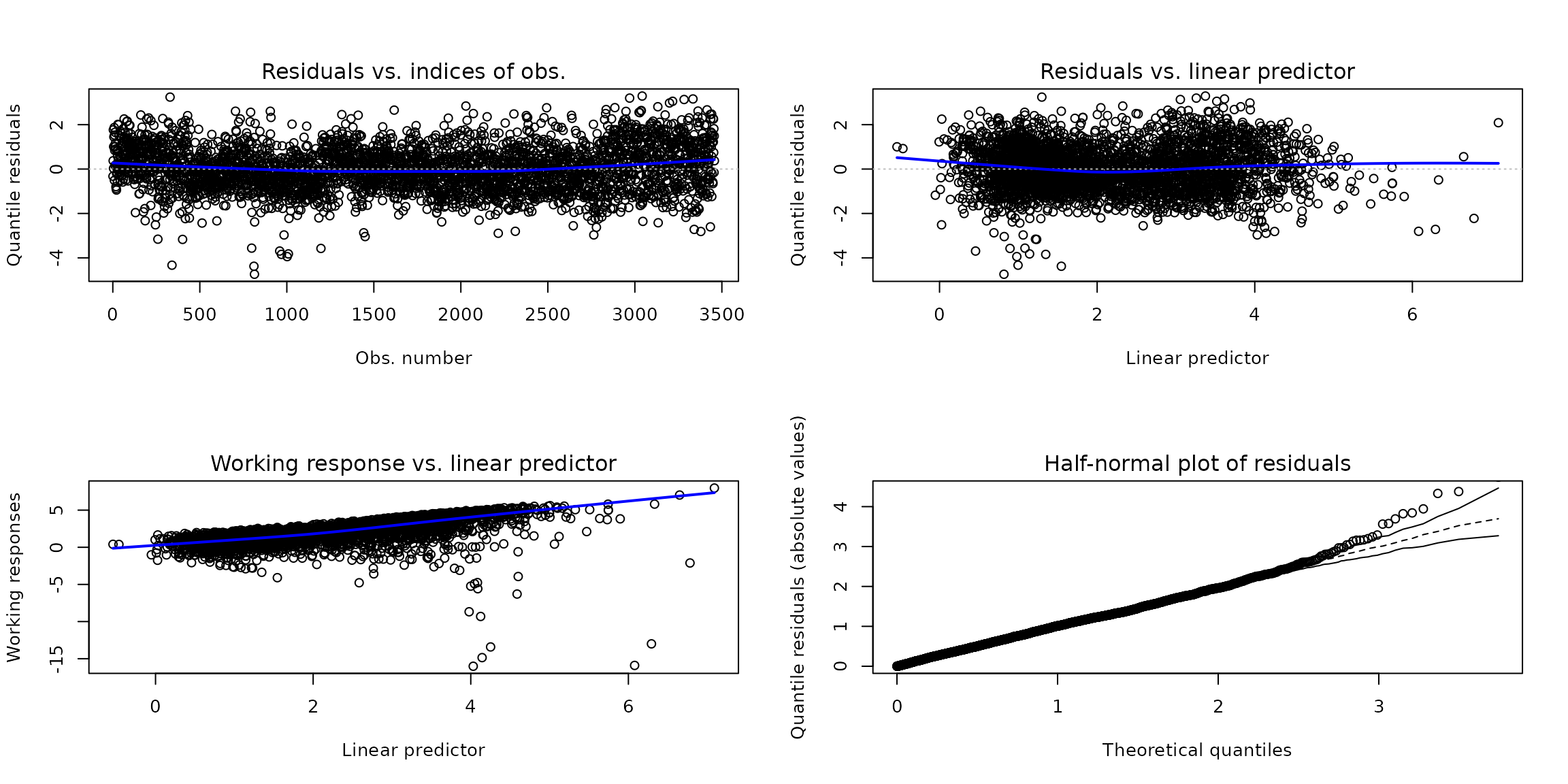
par(oldpar)

Plots of the residuals against the fitted linear predictor and the residuals against indices of observations are the tools for diagnostic analysis to check the structural form of the model. Two features of the plots are important:

Trends: Any trends appearing in these plots indicate that the systematic component can be improved. This could mean changing the link function, adding extra explanatory variables, or transforming the explanatory variables.
Constant variation: If the random component is correct then the variance of the points is approximately constant.

Working residuals versus linear predictor is used to check possible misspecification of link function and Half-normal plot of residuals to check distribution assumption.

Another best practice in diagnostic analysis is to inspect the (Half)-Normal plots with simulated envelope for several quantile value. This is done to obtain a more robust evaluation of the model assumptions. Thus, let’s fit the unit-Logistic quantile regression model for various quantiles.

system.time(
  fits_ulogistic <- unitquantreg(formula = phpws ~ mhdi + incpc + region + log(pop),
                                 data = water, tau = 1:49/50,
                                 family = "ulogistic", link = "logit",
                                 link.theta = "log"))
#>    user  system elapsed 
#>  17.698   4.635  12.906

Now, we can check the (Half)-Normal plots using the output of hnp() method.

library(ggplot2)
get_data <- function(obj) {
  tmp <- hnp(obj, halfnormal = FALSE, plot = FALSE, nsim = 10)
  tmp <- as.data.frame(do.call("cbind", tmp))
  tmp$tau <- as.character(obj$tau)
  tmp
}
chosen_taus <- c("0.02", "0.5", "0.98")
df_plot <- do.call("rbind", lapply(fits_ulogistic[chosen_taus], get_data))
df_plot$tau <- paste0(expression(tau), " == ", df_plot$tau)

ggplot(df_plot, aes(x = teo, y = obs)) +
  facet_wrap(~tau, labeller = label_parsed) +
  geom_point(shape = 3, size = 1.4) +
  geom_line(aes(y = median), linetype = "dashed") +
  geom_line(aes(y = lower), col = "#0080ff") +
  geom_line(aes(y = upper), col = "#0080ff") +
  theme_bw() +
  labs(x = "Theoretical quantiles", y = "Randomized quantile residuals") +
  scale_x_continuous(breaks = seq(-3, 3, by = 1)) +
  scale_y_continuous(breaks = seq(-3, 3, by = 1)) +
  theme_bw() +
  theme(text = element_text(size = 16, family = "Palatino"), 
        panel.grid.minor = element_blank())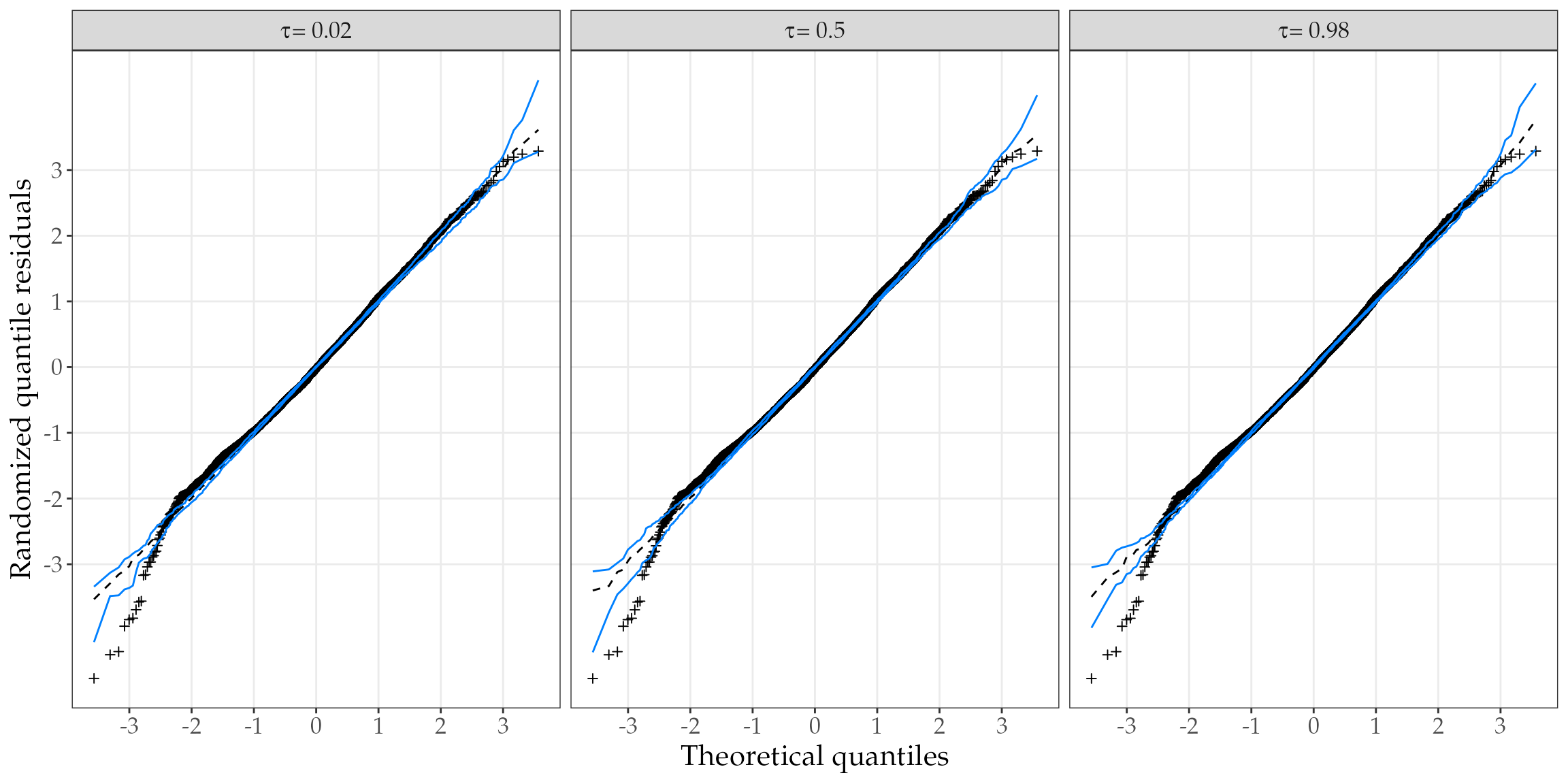

Inference results

Inference results about the parameter estimates can be accessed through the summary method. For instance,

summary(lt_fits[["unit-Logistic"]])
#> 
#>  Wald-tests for unit-Logistic quantile regression model
#> 
#> Call:  unitquantreg(formula = phpws ~ mhdi + incpc + region + log(pop), 
#>     data = water, tau = 0.5, family = fam, link = "logit", link.theta = "log")
#> 
#> Mu coefficients: (quantile model with logit link and tau = 0.5): 
#>               Estimate Std. Error Z value Pr(>|z|)    
#> (Intercept) -5.3654690  0.3373263 -15.906  < 2e-16 ***
#> mhdi        10.5080995  0.5717793  18.378  < 2e-16 ***
#> incpc        0.0015596  0.0001706   9.140  < 2e-16 ***
#> region      -0.1582600  0.0488825  -3.238  0.00121 ** 
#> log(pop)     0.0177337  0.0167306   1.060  0.28917    
#> ---
#> Signif. codes:  0 '***' 0.001 '**' 0.01 '*' 0.05 '.' 0.1 ' ' 1
#> 
#> Model with constant shape:
#>            Estimate Std. Error Z value Pr(>|z|)    
#> log(theta)  0.63006    0.01421   44.35   <2e-16 ***
#> ---
#> Signif. codes:  0 '***' 0.001 '**' 0.01 '*' 0.05 '.' 0.1 ' ' 1
#> 
#> Residual degrees of freedom: 3451
#> Log-likelihood: 4221.514
#> Number of iterations: 63

For unitquantregs objects the plot method provide a convenience to check the significance as well as the effect of estimate along the specify quantile value.

plot(fits_ulogistic, which = "coef")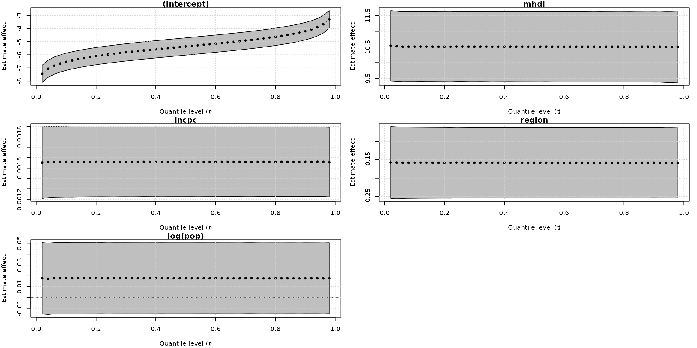

Curiously, the unit-Logistic quantile regression models capture constant effect for all covariates along the different quantiles. In contrast, the unit-Weibull model (the fourth best model) found a decrease effect of mhdi covaraite on the response as the quantile increases and increase effects of incpc and region on the response variable as the quantile increases.

system.time(
  fits_uweibull <- unitquantreg(formula = phpws ~ mhdi + incpc + region + log(pop),
                                 data = water, tau = 1:49/50,
                                 family = "uweibull", link = "logit",
                                 link.theta = "log"))
#>    user  system elapsed 
#>  18.909   4.680  14.013
plot(fits_uweibull, which = "coef")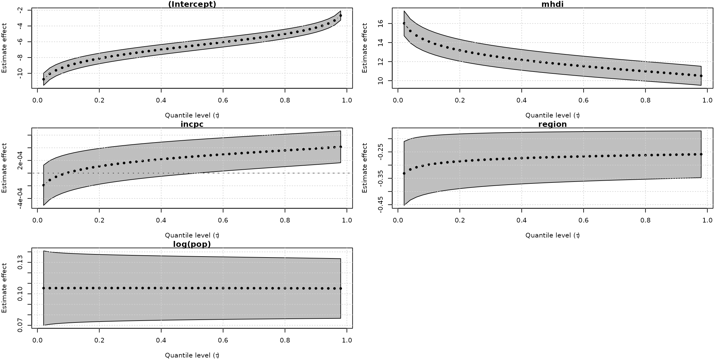

Using the plot() method with argument which = "conddist" for unitquantregs objects it is possible to estimate and visualize the conditional distribution of a response variable at different values of covariates. For instance,

lt_data <- list(mhdi = c(0.5, 0.7), incpc = round(mean(water$incpc)),
                region = c(1, 0), pop = round(mean(water$pop)))
plot(fits_ulogistic, which = "conddist", at_obs = lt_data, at_avg = FALSE,
     dist_type = "density")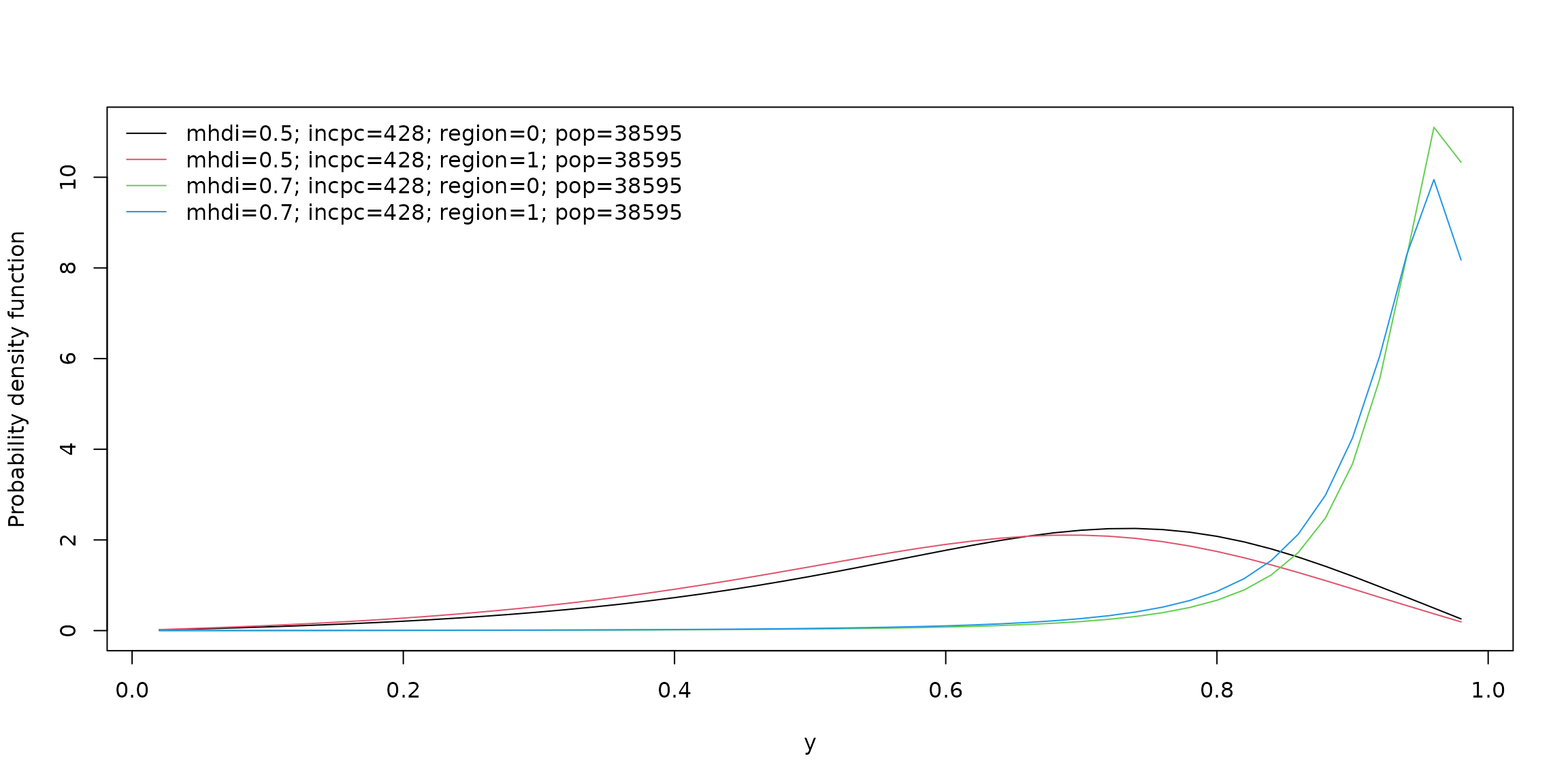

plot(fits_ulogistic, which = "conddist", at_obs = lt_data, at_avg = FALSE,
     dist_type = "cdf")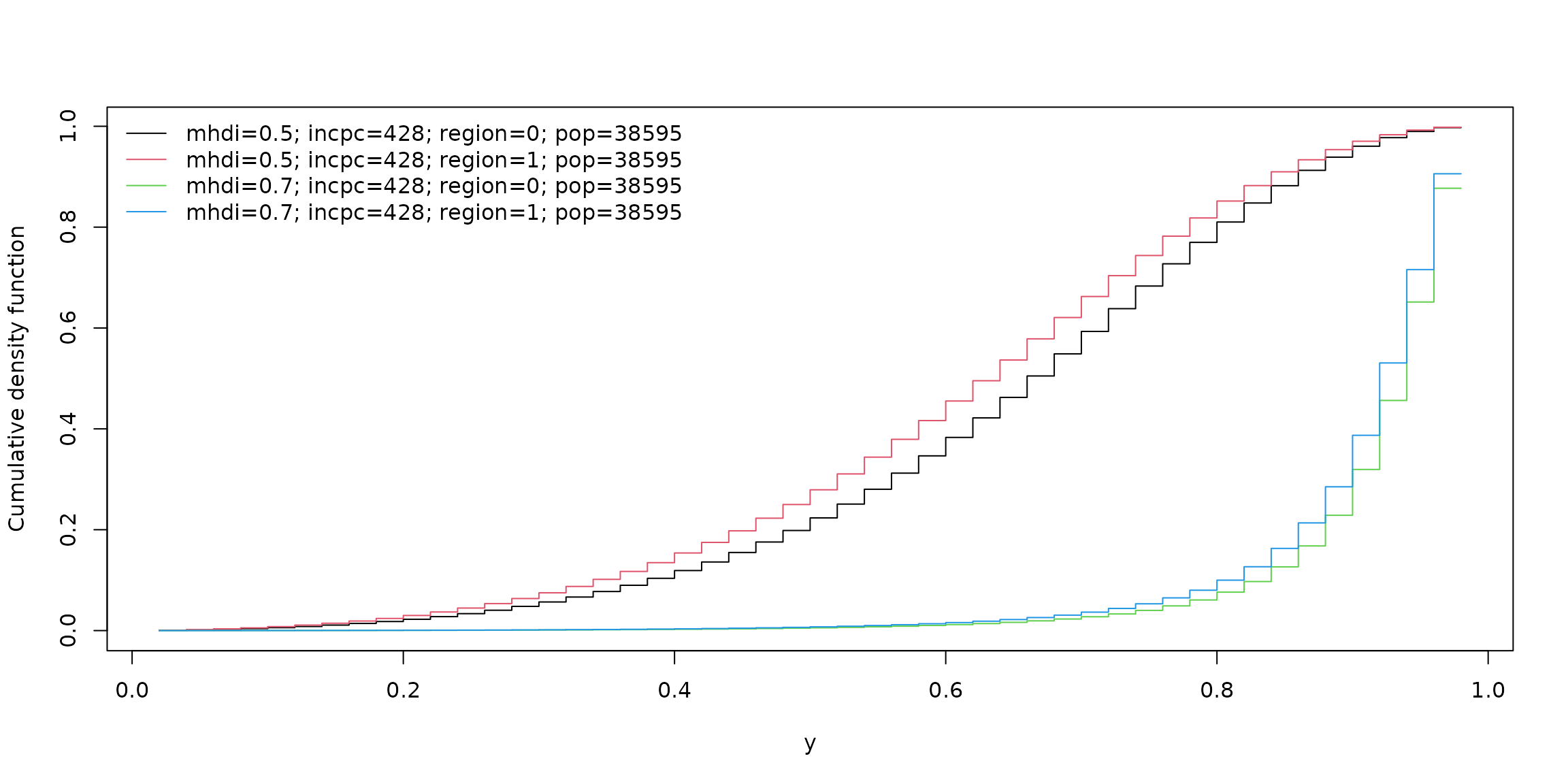

Session info

sessionInfo()
#> R version 4.3.1 (2023-06-16)
#> Platform: x86_64-pc-linux-gnu (64-bit)
#> Running under: Ubuntu 22.04.3 LTS
#> 
#> Matrix products: default
#> BLAS:   /usr/lib/x86_64-linux-gnu/openblas-pthread/libblas.so.3 
#> LAPACK: /usr/lib/x86_64-linux-gnu/openblas-pthread/libopenblasp-r0.3.20.so;  LAPACK version 3.10.0
#> 
#> locale:
#>  [1] LC_CTYPE=C.UTF-8       LC_NUMERIC=C           LC_TIME=C.UTF-8       
#>  [4] LC_COLLATE=C.UTF-8     LC_MONETARY=C.UTF-8    LC_MESSAGES=C.UTF-8   
#>  [7] LC_PAPER=C.UTF-8       LC_NAME=C              LC_ADDRESS=C          
#> [10] LC_TELEPHONE=C         LC_MEASUREMENT=C.UTF-8 LC_IDENTIFICATION=C   
#> 
#> time zone: UTC
#> tzcode source: system (glibc)
#> 
#> attached base packages:
#> [1] stats     graphics  grDevices utils     datasets  methods   base     
#> 
#> other attached packages:
#> [1] ggplot2_3.4.3      unitquantreg_0.0.6
#> 
#> loaded via a namespace (and not attached):
#>  [1] utf8_1.2.3          sass_0.4.7          stringi_1.7.12     
#>  [4] lattice_0.21-8      pracma_2.4.2        digest_0.6.33      
#>  [7] magrittr_2.0.3      evaluate_0.21       grid_4.3.1         
#> [10] fastmap_1.1.1       rprojroot_2.0.3     jsonlite_1.8.7     
#> [13] Matrix_1.6-1        Formula_1.2-5       survival_3.5-7     
#> [16] fansi_1.0.4         purrr_1.0.2         scales_1.2.1       
#> [19] codetools_0.2-19    numDeriv_2016.8-1.1 textshaping_0.3.6  
#> [22] jquerylib_0.1.4     cli_3.6.1           rlang_1.1.1        
#> [25] munsell_0.5.0       splines_4.3.1       withr_2.5.0        
#> [28] cachem_1.0.8        yaml_2.3.7          tools_4.3.1        
#> [31] SparseM_1.81        MatrixModels_0.5-2  memoise_2.0.1      
#> [34] nloptr_2.0.3        colorspace_2.1-0    optimx_2023-8.13   
#> [37] vctrs_0.6.3         R6_2.5.1            lifecycle_1.0.3    
#> [40] stringr_1.5.0       fs_1.6.3            MASS_7.3-60        
#> [43] ragg_1.2.5          pkgconfig_2.0.3     desc_1.4.2         
#> [46] pillar_1.9.0        pkgdown_2.0.7       bslib_0.5.1        
#> [49] gtable_0.3.4        glue_1.6.2          Rcpp_1.0.11        
#> [52] systemfonts_1.0.4   xfun_0.40           tibble_3.2.1       
#> [55] knitr_1.44          farver_2.1.1        htmltools_0.5.6    
#> [58] rmarkdown_2.24      compiler_4.3.1      quantreg_5.97

André Menezes

Last compiled on 2023-09-12