Density function, distribution function, quantile function and random number generation for the Kumaraswamy distribution reparametrized in terms of the \(\tau\)-th quantile, \(\tau \in (0, 1)\).
Usage
dkum(x, mu, theta, tau = 0.5, log = FALSE)

pkum(q, mu, theta, tau = 0.5, lower.tail = TRUE, log.p = FALSE)

qkum(p, mu, theta, tau = 0.5, lower.tail = TRUE, log.p = FALSE)

rkum(n, mu, theta, tau = 0.5)
Arguments
- x, q
vector of positive quantiles.
- mu
location parameter indicating the \(\tau\)-th quantile, \(\tau \in (0, 1)\).
- theta
nonnegative shape parameter.
- tau
the parameter to specify which quantile is to used.
- log, log.p
logical; If TRUE, probabilities p are given as log(p).
- lower.tail
logical; If TRUE, (default), \(P(X \leq{x})\) are returned, otherwise \(P(X > x)\).
- p
vector of probabilities.
- n
number of observations. If
length(n) > 1, the length is taken to be the number required.
Value
dkum gives the density, pkum gives the distribution function,
qkum gives the quantile function and rkum generates random deviates.
Invalid arguments will return an error message.
Details
Probability density function $$f(y\mid \alpha ,\theta )=\alpha \theta y^{\theta -1}(1-y^{\theta })^{\alpha-1}$$
Cumulative distribution function $$F(y\mid \alpha ,\theta )=1-\left( 1-y^{\theta }\right) ^{\alpha }$$
Quantile function $$Q(\tau \mid \alpha ,\theta )=\left[ 1-\left( 1-\tau \right) ^{\frac{1}{\alpha }}\right] ^{\frac{1}{\theta }}$$
Reparameterization $$\alpha=g^{-1}(\mu )=\frac{\log (1-\tau )}{\log (1-\mu ^{\theta })}$$
References
Kumaraswamy, P., (1980). A generalized probability density function for double-bounded random processes. Journal of Hydrology, 46(1), 79--88.
Jones, M. C., (2009). Kumaraswamy's distribution: A beta-type distribution with some tractability advantages. Statistical Methodology, 6(1), 70-81.
Examples
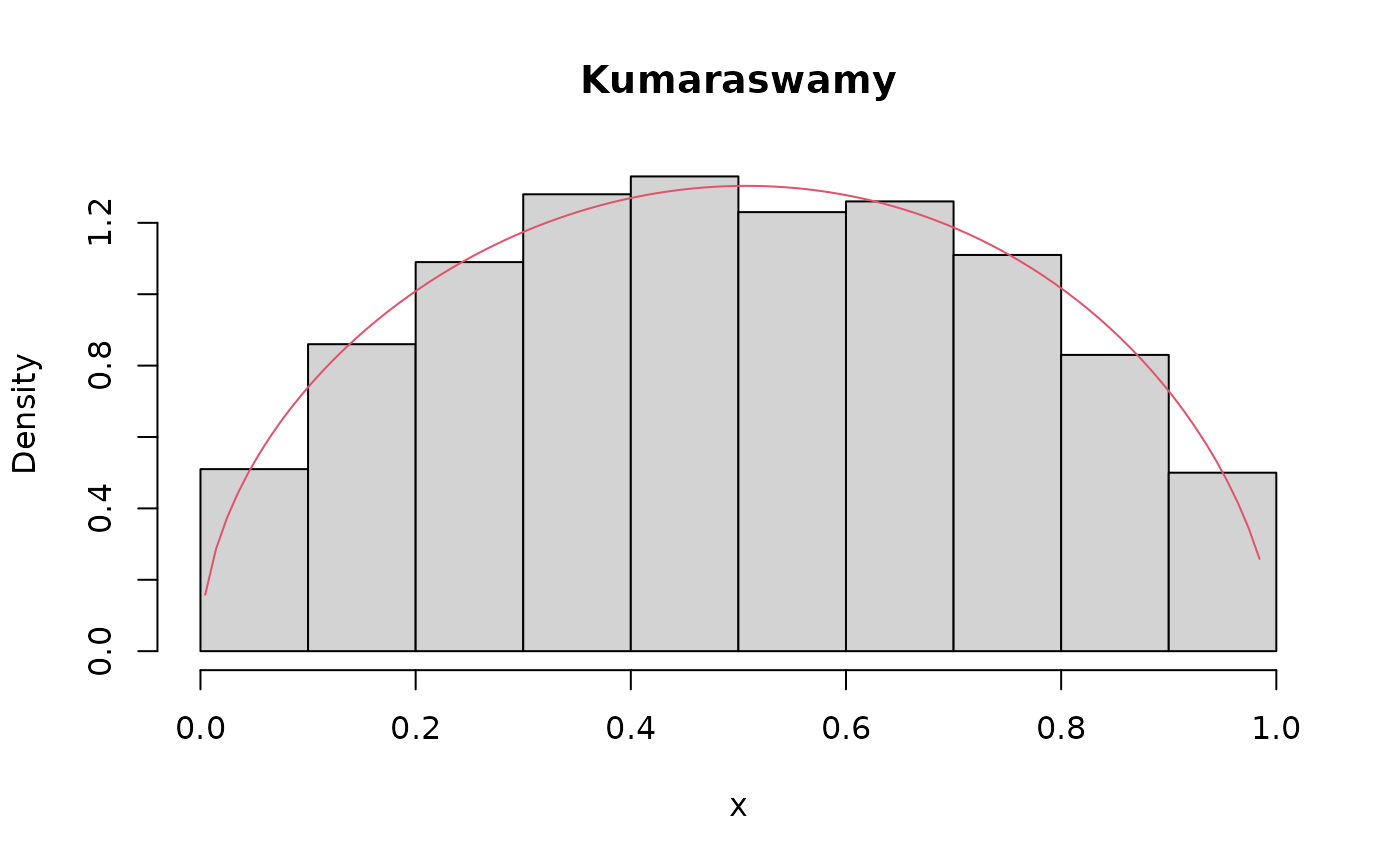
set.seed(123)
x <- rkum(n = 1000, mu = 0.5, theta = 1.5, tau = 0.5)
R <- range(x)
S <- seq(from = R[1], to = R[2], by = 0.01)
hist(x, prob = TRUE, main = 'Kumaraswamy')
lines(S, dkum(x = S, mu = 0.5, theta = 1.5, tau = 0.5), col = 2)
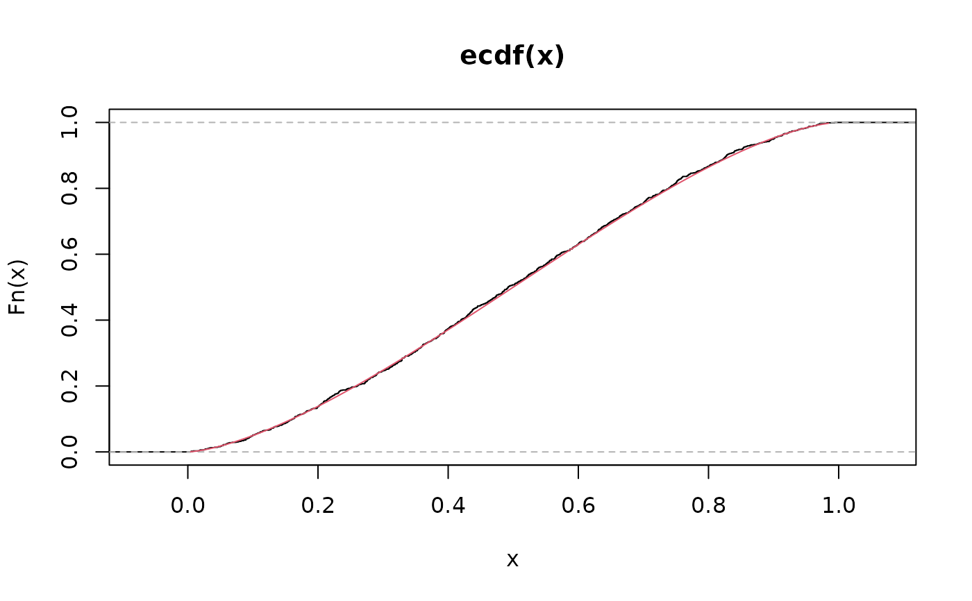
 plot(ecdf(x))
lines(S, pkum(q = S, mu = 0.5, theta = 1.5, tau = 0.5), col = 2)
plot(ecdf(x))
lines(S, pkum(q = S, mu = 0.5, theta = 1.5, tau = 0.5), col = 2)
 plot(quantile(x, probs = S), type = "l")
lines(qkum(p = S, mu = 0.5, theta = 1.5, tau = 0.5), col = 2)
plot(quantile(x, probs = S), type = "l")
lines(qkum(p = S, mu = 0.5, theta = 1.5, tau = 0.5), col = 2)