Density function, distribution function, quantile function and random number generation function for the unit-Birnbaum-Saunders distribution reparametrized in terms of the \(\tau\)-th quantile, \(\tau \in (0, 1)\).
Usage
dubs(x, mu, theta, tau = 0.5, log = FALSE)

pubs(q, mu, theta, tau = 0.5, lower.tail = TRUE, log.p = FALSE)

qubs(p, mu, theta, tau = 0.5, lower.tail = TRUE, log.p = FALSE)

rubs(n, mu, theta, tau = 0.5)
Arguments
- x, q
vector of positive quantiles.
- mu
location parameter indicating the \(\tau\)-th quantile, \(\tau \in (0, 1)\).
- theta
nonnegative shape parameter.
- tau
the parameter to specify which quantile is to be used.
- log, log.p
logical; If TRUE, probabilities p are given as log(p).
- lower.tail
logical; If TRUE, (default), \(P(X \leq{x})\) are returned, otherwise \(P(X > x)\).
- p
vector of probabilities.
- n
number of observations. If
length(n) > 1, the length is taken to be the number required.
Value
dubs gives the density, pubs gives the distribution function,
qubs gives the quantile function and rubs generates random deviates.
Invalid arguments will return an error message.
Details
Probability density function $$f(y\mid \alpha ,\theta )=\frac{1}{2y\alpha \theta \sqrt{2\pi }}\left[\left( -\frac{\alpha }{\log (y)}\right) ^{\frac{1}{2}}+\left( -\frac{\alpha}{\log (y)}\right) ^{\frac{3}{2}}\right] \exp \left[ \frac{1}{2\theta ^{2}}\left( 2+\frac{\log (y)}{\alpha }+\frac{\alpha }{\log (y)}\right) \right]$$
Cumulative distribution function $$F(y\mid \alpha ,\theta )=1-\Phi \left\{ \frac{1}{\theta }\left[ \left( -\frac{\log (y)}{\alpha }\right) ^{\frac{1}{2}}-\left( -\frac{\alpha }{\log(y)}\right) ^{\frac{1}{2}}\right] \right\}$$
Quantile function $$Q\left( \tau \mid \alpha ,\theta \right) ={\exp }\left\{ -{\frac{2\alpha}{2+\left[ {\theta }\Phi ^{-1}\left( 1-\tau \right) \right] ^{2}-{\theta } \Phi ^{-1}\left( 1-\tau \right) \sqrt{4+\left[ {\theta }\Phi ^{-1}\left(1-\tau \right) \right] ^{2}}}}\right\}$$
Reparameterization $$\alpha=g^{-1}(\mu )=\log \left( \mu \right) g\left( \theta ,\tau \right)$$ where \(g\left( \theta ,\tau \right) =-\frac{1}{2}\left\{ 2+\left[ {\theta }\Phi^{-1}\left( 1-\tau \right) \right] ^{2}-{\theta }\Phi ^{-1}\left( 1-\tau\right) \sqrt{4+{\theta }\Phi ^{-1}\left( 1-\tau \right) }\right\} .\)
References
Birnbaum, Z. W. and Saunders, S. C., (1969). A new family of life distributions. Journal of Applied Probability, 6(2), 637--652. Mazucheli, J., Menezes, A. F. B. and Dey, S., (2018). The unit-Birnbaum-Saunders distribution with applications. Chilean Journal of Statistics, 9(1), 47--57.
Mazucheli, J., Alves, B. and Menezes, A. F. B., (2021). A new quantile regression for modeling bounded data under a unit Birnbaum-Saunders distribution with applications. Simmetry, (), 1--28.
Examples
set.seed(123)
x <- rubs(n = 1000, mu = 0.5, theta = 1.5, tau = 0.5)
R <- range(x)
S <- seq(from = R[1], to = R[2], by = 0.01)
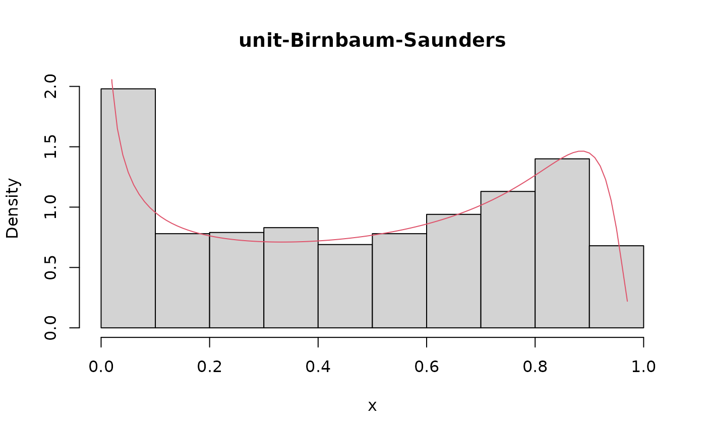
hist(x, prob = TRUE, main = 'unit-Birnbaum-Saunders')
lines(S, dubs(x = S, mu = 0.5, theta = 1.5, tau = 0.5), col = 2)
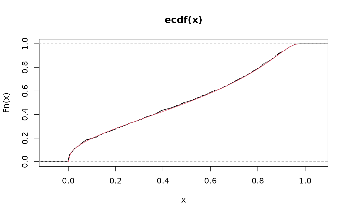
 plot(ecdf(x))
lines(S, pubs(q = S, mu = 0.5, theta = 1.5, tau = 0.5), col = 2)
plot(ecdf(x))
lines(S, pubs(q = S, mu = 0.5, theta = 1.5, tau = 0.5), col = 2)
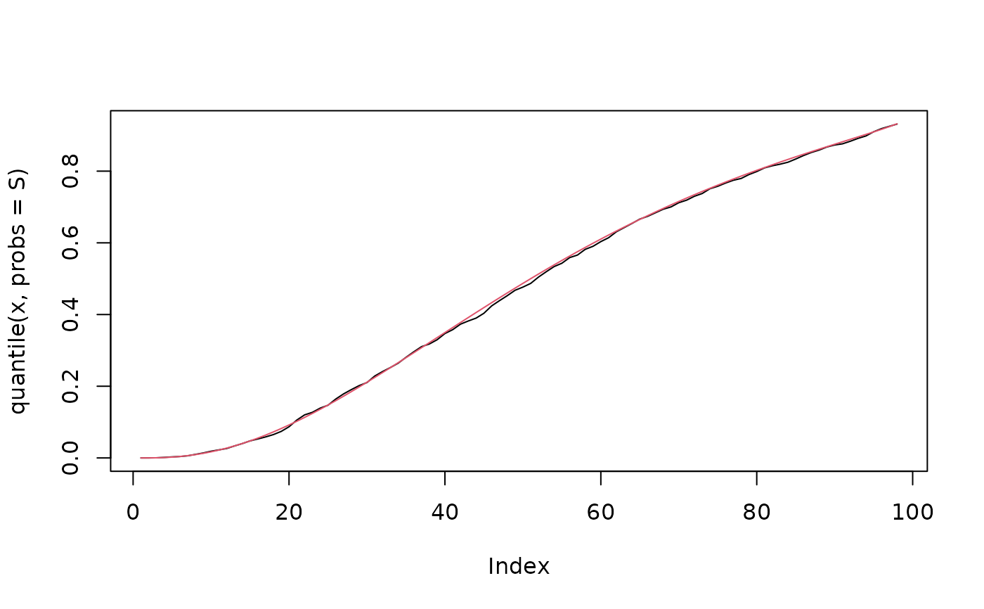
 plot(quantile(x, probs = S), type = "l")
lines(qubs(p = S, mu = 0.5, theta = 1.5, tau = 0.5), col = 2)
plot(quantile(x, probs = S), type = "l")
lines(qubs(p = S, mu = 0.5, theta = 1.5, tau = 0.5), col = 2)