Density function, distribution function, quantile function and random number generation function for the unit-Half-Normal-E distribution reparametrized in terms of the \(\tau\)-th quantile, \(\tau \in (0, 1)\).
Usage
dughne(x, mu, theta, tau = 0.5, log = FALSE)

pughne(q, mu, theta, tau = 0.5, lower.tail = TRUE, log.p = FALSE)

qughne(p, mu, theta, tau = 0.5, lower.tail = TRUE, log.p = FALSE)

rughne(n, mu, theta, tau = 0.5)
Arguments
- x, q
vector of positive quantiles.
- mu
location parameter indicating the \(\tau\)-th quantile, \(\tau \in (0, 1)\).
- theta
nonnegative shape parameter.
- tau
the parameter to specify which quantile is to be used.
- log, log.p
logical; If TRUE, probabilities p are given as log(p).
- lower.tail
logical; If TRUE, (default), \(P(X \leq{x})\) are returned, otherwise \(P(X > x)\).
- p
vector of probabilities.
- n
number of observations. If
length(n) > 1, the length is taken to be the number required.
Value
dughne gives the density, pughne gives the distribution function,
qughne gives the quantile function and rughne generates random deviates.
Invalid arguments will return an error message.
Details
Probability density function $$f(y\mid \alpha ,\theta )=\sqrt{\frac{2}{\pi }}\frac{\theta }{y\left[ -\log\left( y\right) \right] }\left( -{\frac{\log \left( y\right) }{\alpha }} \right)^{\theta }\mathrm{\exp }\left\{ -\frac{1}{2}\left[ -{\frac{\log \left( y\right) }{\alpha }}\right]^{2\theta }\right\}$$
Cumulative distribution function $$F(y\mid \alpha ,\theta )=2\Phi \left[ -\left( -{\frac{\log \left( y\right) }{\alpha }}\right)^{\theta }\right]$$
Quantile function $$Q(\tau \mid \alpha ,\theta )=\exp \left\{ -\alpha \left[ -\Phi^{-1}\left(\frac{\tau }{2}\right) \right]^{\frac{1}{\theta }}\right\}$$
Reparameterization $$\alpha=g^{-1}(\mu )=-\log \left( \mu \right) \left[ -\Phi^{-1}\left( \frac{\tau }{2}\right) \right]^{-\frac{1}{\theta }}$$
References
Korkmaz, M. C., (2020). The unit generalized half normal distribution: A new bounded distribution with inference and application. University Politehnica of Bucharest Scientific, 82(2), 133--140.
Examples
set.seed(123)
x <- rughne(n = 1000, mu = 0.5, theta = 2, tau = 0.5)
R <- range(x)
S <- seq(from = R[1], to = R[2], by = 0.01)
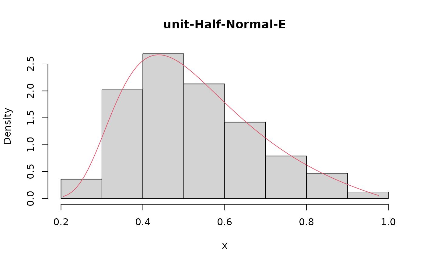
hist(x, prob = TRUE, main = 'unit-Half-Normal-E')
lines(S, dughne(x = S, mu = 0.5, theta = 2, tau = 0.5), col = 2)
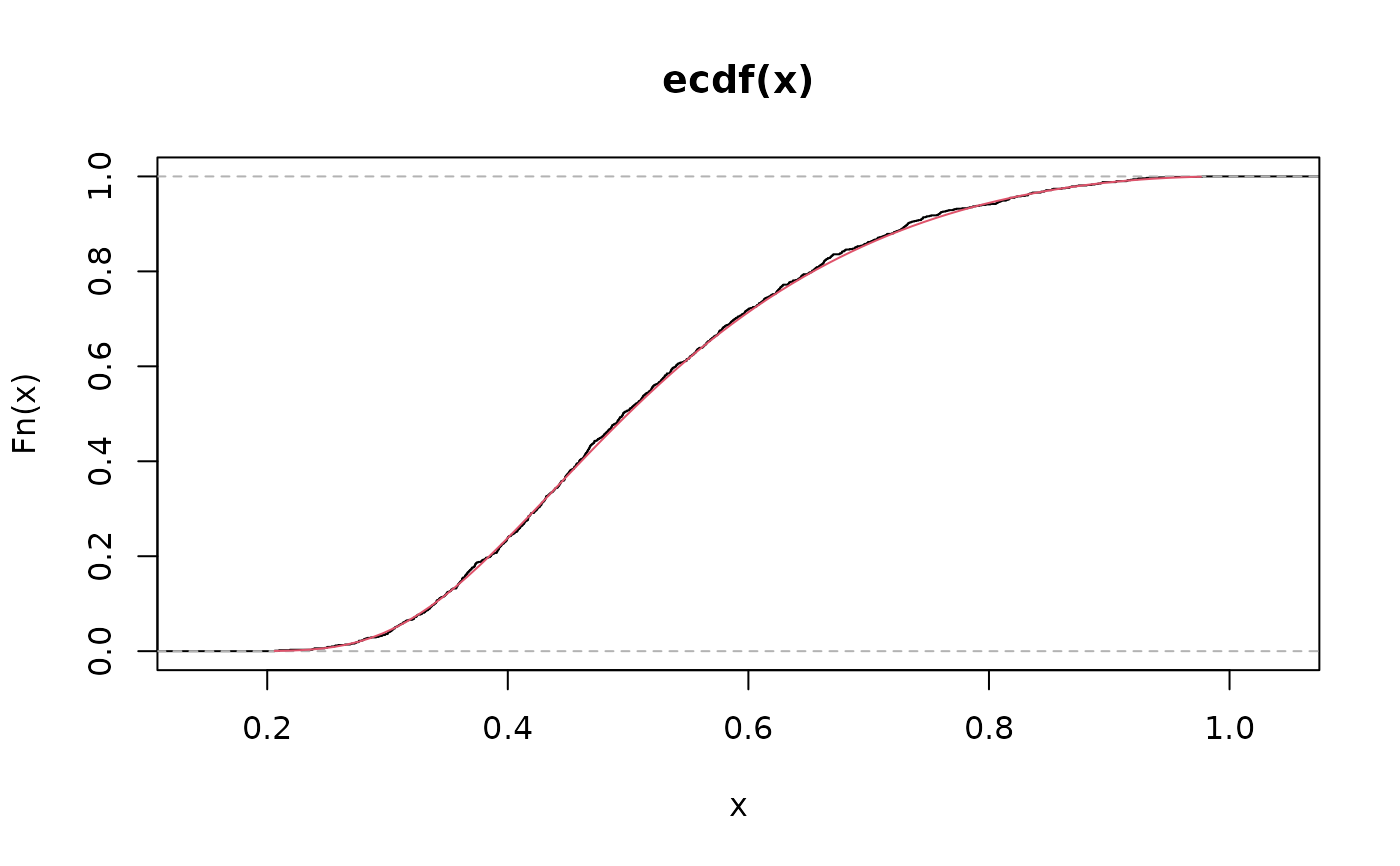
 plot(ecdf(x))
lines(S, pughne(q = S, mu = 0.5, theta = 2, tau = 0.5), col = 2)
plot(ecdf(x))
lines(S, pughne(q = S, mu = 0.5, theta = 2, tau = 0.5), col = 2)
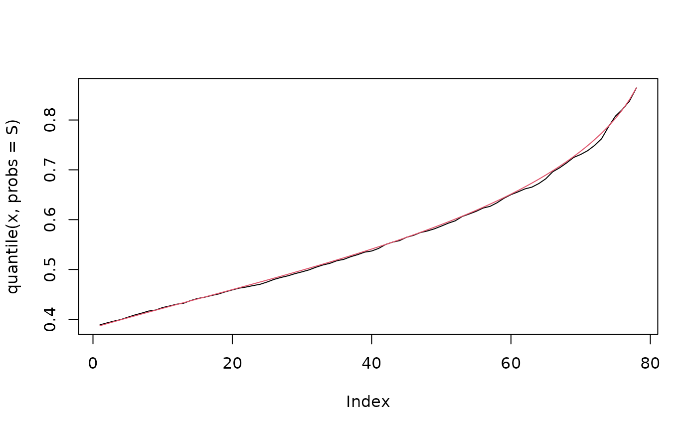
 plot(quantile(x, probs = S), type = "l")
lines(qughne(p = S, mu = 0.5, theta = 2, tau = 0.5), col = 2)
plot(quantile(x, probs = S), type = "l")
lines(qughne(p = S, mu = 0.5, theta = 2, tau = 0.5), col = 2)