Density function, distribution function, quantile function and random number generation for the unit-Logistic distribution reparametrized in terms of the \(\tau\)-th quantile, \(\tau \in (0, 1)\).
Usage
dulogistic(x, mu, theta, tau = 0.5, log = FALSE)

pulogistic(q, mu, theta, tau = 0.5, lower.tail = TRUE, log.p = FALSE)

qulogistic(p, mu, theta, tau = 0.5, lower.tail = TRUE, log.p = FALSE)

rulogistic(n, mu, theta, tau = 0.5)
Arguments
- x, q
vector of positive quantiles.
- mu
location parameter indicating the \(\tau\)-th quantile, \(\tau \in (0, 1)\).
- theta
nonnegative shape parameter.
- tau
the parameter to specify which quantile is to used.
- log, log.p
logical; If TRUE, probabilities p are given as log(p).
- lower.tail
logical; If TRUE, (default), \(P(X \leq{x})\) are returned, otherwise \(P(X > x)\).
- p
vector of probabilities.
- n
number of observations. If
length(n) > 1, the length is taken to be the number required.
Value
dulogistic gives the density, pulogistic gives the distribution function,
qulogistic gives the quantile function and rulogistic generates random deviates.
Invalid arguments will return an error message.
Details
Probability density function $$f(y\mid \alpha ,\theta )=\frac{\theta \exp \left( \alpha \right) \left(\frac{y}{1-y}\right) ^{\theta -1}}{\left[ 1+\exp \left( \alpha \right)\left( \frac{y}{1-y}\right) ^{\theta }\right] ^{2}}$$
Cumulative distribution function $$F(y\mid \alpha ,\theta )=\frac{\exp \left( \alpha \right) \left( \frac{y}{1-y}\right) ^{\theta }}{1+\exp \left( \alpha \right) \left( \frac{y}{1-y}\right) ^{\theta }}$$
Quantile function $$Q(\tau \mid \alpha ,\theta )=\frac{\exp \left( -\frac{\alpha }{\theta }\right) \left( \frac{\tau }{1-\tau }\right) ^{\frac{1}{\theta }}}{1+\exp\left( -\frac{\alpha }{\theta }\right) \left( \frac{\tau }{1-\tau }\right) ^{ \frac{1}{\theta }}} $$
Reparameterization $$\alpha=g^{-1}(\mu )=\log \left( \frac{\tau }{1-\tau }\right) -\theta \log \left( \frac{\mu }{1-\mu }\right) $$
References
Paz, R. F., Balakrishnan, N. and Bazán, J. L., 2019. L-Logistic regression models: Prior sensitivity analysis, robustness to outliers and applications. Brazilian Journal of Probability and Statistics, 33(3), 455--479.
Examples
set.seed(123)
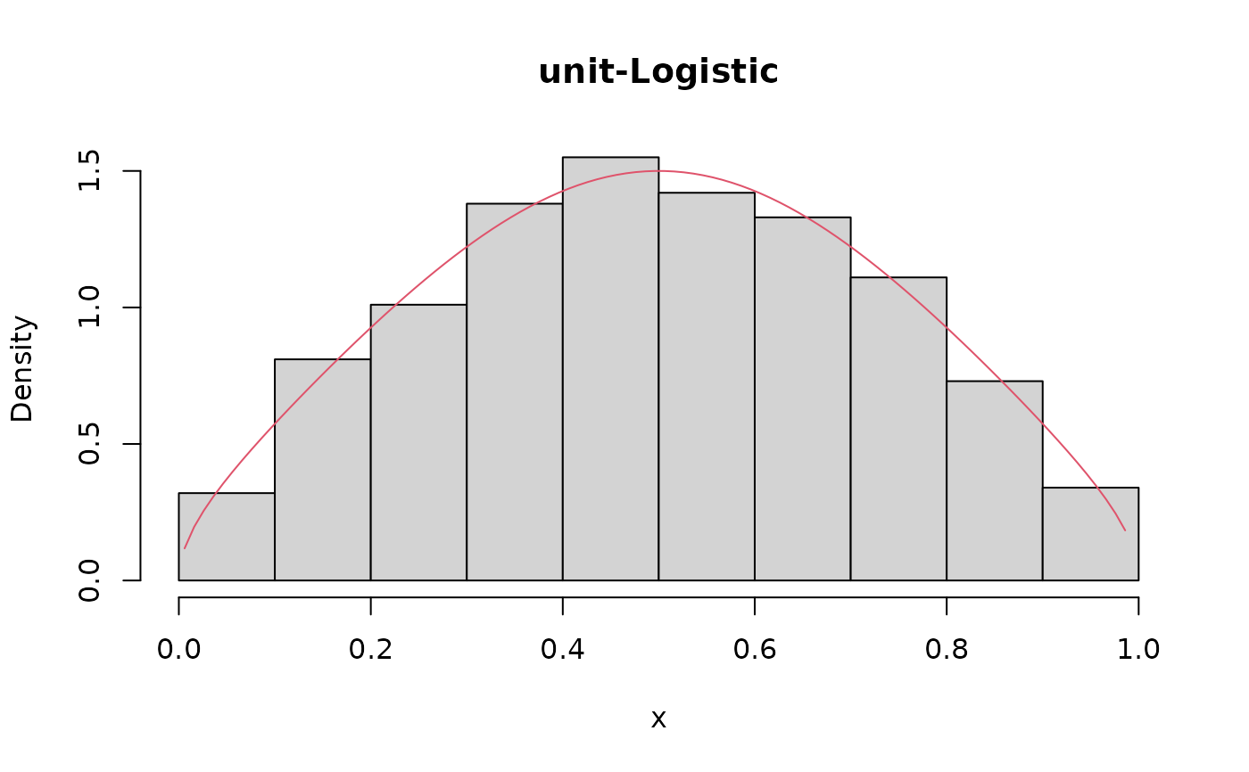
x <- rulogistic(n = 1000, mu = 0.5, theta = 1.5, tau = 0.5)
R <- range(x)
S <- seq(from = R[1], to = R[2], by = 0.01)
hist(x, prob = TRUE, main = 'unit-Logistic')
lines(S, dulogistic(x = S, mu = 0.5, theta = 1.5, tau = 0.5), col = 2)
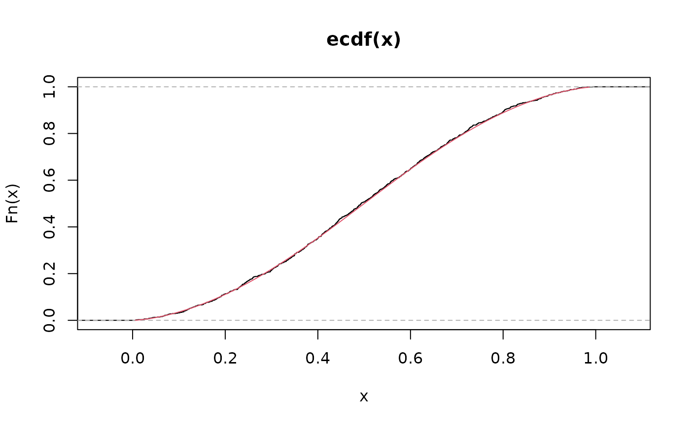
 plot(ecdf(x))
lines(S, pulogistic(q = S, mu = 0.5, theta = 1.5, tau = 0.5), col = 2)
plot(ecdf(x))
lines(S, pulogistic(q = S, mu = 0.5, theta = 1.5, tau = 0.5), col = 2)
 plot(quantile(x, probs = S), type = "l")
lines(qulogistic(p = S, mu = 0.5, theta = 1.5, tau = 0.5), col = 2)
plot(quantile(x, probs = S), type = "l")
lines(qulogistic(p = S, mu = 0.5, theta = 1.5, tau = 0.5), col = 2)